
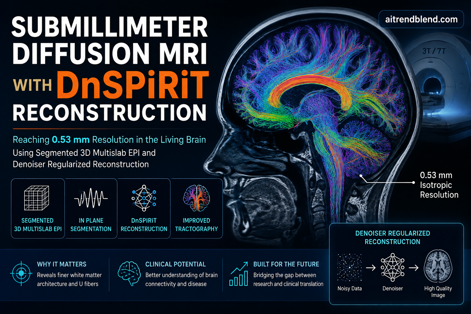
Push a diffusion MRI scanner hard enough and the brain starts to give up secrets it normally hides. Most clinical and research diffusion scans work at roughly one to two millimeters per voxel, which sounds fine until you remember that a cortical gyrus can fold, turn, and send fibers into a sulcal wall inside a space smaller than that. At that scale the scan blurs two stories into one. A team at the University of Oxford went after the resolution barrier directly and pulled living human brain diffusion data down to 0.53 mm.
Read this first
This article explains published research. It is not medical advice, diagnosis, or treatment. The work described here is a methods study in healthy volunteers and has not been validated as a clinical tool. Anyone with questions about brain imaging or a neurological condition should consult a qualified clinician.
Key points
- Oxford researchers acquired in vivo brain diffusion MRI at 0.53 mm and 0.65 mm on a standard 3T scanner and 0.61 mm at 7T, well past the usual clinical resolution near 1 to 2 mm.
- The gains come from two changes working together, an in plane segmented 3D multislab acquisition that shortens echo spacing and echo time, and a reconstruction called DnSPIRiT that folds a denoiser into the image estimate rather than blurring it in afterward.
- DnSPIRiT lifted signal to noise ratio by about 66 percent over a plain reconstruction while cutting the sharpness loss of standalone denoising roughly in half, and it matched a reference scan for diffusion metrics more closely than either alternative.
- At high resolution the data reduced the well known gyral bias and resolved short association fibers, the U fibers, even where they arc sharply around a fold.
- The whole pipeline runs on Pulseq, an open and scanner agnostic sequence framework, which lowers the barrier for other labs to reproduce it.
- This is a small study in a handful of volunteers, so the clinical payoff remains a promise rather than a result.
Why one millimeter is not good enough
The problem runs deeper than it first appears. Diffusion MRI maps the direction water tends to move inside tissue, and in white matter that direction follows the axon bundles. Trace those directions voxel by voxel and you can reconstruct fiber pathways, the raw material of brain connectivity maps. The catch is that a tractography algorithm can only follow what the voxel grid resolves. When a voxel is 1.22 mm on a side and a bundle turns inside that voxel, the turn averages out and the algorithm marches straight through it.
Two anatomical phenomena suffer most from this. The first is gyral bias, a stubborn artifact where reconstructed streamlines pile up at the crowns of the cortical folds and rarely reach the walls of the sulci between them. Real axons fan out to cover both. The second is the family of short association fibers just under the cortex, called U fibers because they dip down from one gyrus and loop back up to the neighbor. Those fibers make up the majority of the brain’s axonal connections and they are among the first to degrade in diseases such as Alzheimer’s. A scan that cannot see them cannot study them.
Postmortem work had already shown what submillimeter diffusion imaging reveals, because a fixed brain can sit in a scanner for many hours. Doing it in a living person is a different fight. Small voxels hold fewer water molecules, so they return a weaker signal, and the signal to noise ratio in diffusion imaging falls fast as voxels shrink. Worse, the standard readout method, echo planar imaging, needs longer echo trains to encode a bigger image matrix. Longer readouts mean more distortion, more blurring from T2* decay, and longer echo times that let the diffusion signal fade before it is even measured. Everything you do to chase resolution tends to wreck the image you were trying to sharpen.
The acquisition side, segmenting the readout in the plane
The Oxford group, Ziyu Li, Silei Zhu, Karla L. Miller, and Wenchuan Wu at the Oxford Centre for Integrative Neuroimaging, started from a known strong foundation and reshaped it. That foundation is 3D multislab imaging, which excites a thick slab and encodes it in three dimensions rather than slice by slice. Multislab acquisition has the best signal to noise efficiency of the practical options because it collects signal from a whole slab at once and works well at the repetition times diffusion imaging likes. Its weakness is that a single shot readout across a full plane at submillimeter resolution takes a long time, which brings back the long echo time and the blurring.
Their fix is in plane segmentation. Instead of covering one plane of the encoding grid in a single shot, they split the phase encoding into several interleaved segments and acquire each with a shorter readout. Six segments at 0.53 mm and 0.65 mm on the 3T scanner, eight at 0.61 mm on the 7T scanner. Shorter readouts mean shorter effective echo spacing, and the numbers are striking. The effective echo spacing dropped to about 0.21 ms at 0.65 mm and 0.15 ms at 0.61 mm. Short echo spacing is the lever that controls distortion and T2* blurring, so shrinking it is exactly what a high resolution protocol needs.
Before touching a scanner the team ran numerical simulations to justify the design. They modeled how effective resolution and signal to noise ratio respond to the number of segments, to partial Fourier sampling, and to field strength, using realistic white matter relaxation values at 3T and 7T. Those simulations are where the six and eight segment choices came from rather than guesswork. The simulated signal to noise ratio follows a relationship worth showing, because it makes the tradeoffs explicit.
Read that expression as a budget. Signal to noise ratio climbs steeply with field strength \(B_0\), which is why 7T helps so much. It scales with the voxel volume \(\Delta x \Delta y \Delta z\), which is the whole reason small voxels hurt. And it falls with the \(e^{-TE/T_2}\) term, so any reduction in echo time earned by shorter readouts pays off directly in retained signal. In plane segmentation buys back signal on that last term even as the voxel shrinks. To keep the whole thing portable, the sequences were built in Pulseq, an open framework that runs across scanner vendors, which matters because a method nobody else can install tends to stay in one lab.
A shorter readout is not a cosmetic tweak. It is the difference between measuring the diffusion signal and measuring what is left of it after the brain has stopped talking. On the role of effective echo spacing in submillimeter diffusion MRI
The reconstruction side, a denoiser that lives inside the estimate
Better acquisition still leaves noisy images, so the second half of the paper is about reconstruction. Here is where it gets interesting. The obvious move is to reconstruct the image with a standard parallel imaging method and then run a denoiser over the result. The team calls this SPIRiT followed by standalone denoising, and it does raise signal to noise ratio dramatically. It also smears fine structure, because a denoiser applied after the fact has no memory of the measured data and will happily erase real anatomy along with the noise.
Their answer is DnSPIRiT, short for denoiser regularized SPIRiT. Rather than denoise at the end, they write the denoiser into the reconstruction as a regularizer and solve for the image that stays faithful to the acquired k space, respects the coil calibration, and looks like a denoised image, all at once. The objective they minimize captures those three demands.
The first term is data fidelity. It says the reconstructed k space \(x\), once sampled by each shot’s mask \(D_i\) and adjusted for that shot’s motion induced phase \(P_i\), has to match the acquired data \(y_i\). The second term uses the SPIRiT kernel \(G\) learned from coil calibration data to enforce consistency across receive channels. The third term is the new one. It penalizes the distance between the image and its denoised version \(\Phi\), with \(\Phi\) being an off the shelf denoiser. Because the denoiser only ever pulls the estimate toward a cleaner image while the data term holds it to the measurements, the reconstruction gains the noise suppression without drifting away from the truth.
They solve it with a plug and play scheme that alternates between a reconstruction step and a denoising step, five iterations for the six direction protocols and two for the twenty direction protocol. The denoiser itself is swapped depending on the data. For the six direction 3T and 7T protocols they used BM4D, an image space block matching denoiser. For the twenty direction 0.53 mm protocol they used NORDIC, a complex denoiser that works well when there are enough diffusion volumes to estimate the noise. The framework does not care which denoiser you drop in, which is part of the appeal.
What the numbers actually show
The team compared three reconstructions on the same 3T 0.65 mm data, plain SPIRiT, SPIRiT with standalone denoising, and DnSPIRiT. They measured signal to noise ratio on the non diffusion image and on the diffusion weighted images, angular contrast to noise ratio, image sharpness through a normalized Tenengrad focus measure, and the bias in two standard diffusion metrics relative to a 1.22 mm reference, fractional anisotropy and mean diffusivity. The table below is the heart of the comparison.
| Method | SNR b=0 | SNR DWI | CNR DWI | Sharpness | |ΔFA| | |ΔMD| (×10⁻⁵ mm²/s) |
|---|---|---|---|---|---|---|
| SPIRiT | 6.65 | 3.18 | 0.87 | 0.50 | 0.163 | 4.54 |
| SPIRiT + denoising | 13.45 | 6.25 | 1.17 | 0.28 | 0.019 | 3.85 |
| DnSPIRiT | 11.19 | 5.29 | 1.04 | 0.39 | 0.002 | 3.62 |
The numbers tell a complicated story, which is exactly why they are worth reading carefully. Standalone denoising wins the raw signal to noise ratio and contrast columns outright, roughly doubling signal to noise ratio over plain SPIRiT. If those were the only columns that mattered you would stop there. They are not. Look at sharpness. Plain SPIRiT holds sharpness at 0.50, standalone denoising collapses it to 0.28, a 44 percent loss, and DnSPIRiT lands at 0.39, only about a 22 percent loss. DnSPIRiT keeps most of the signal to noise gain, about 66 percent above plain SPIRiT, while giving back only half the sharpness that the naive approach throws away.
Then look at the bias columns, which are the ones a scientist should care about most, because a diffusion metric that is precise but wrong is a trap. DnSPIRiT posts an absolute fractional anisotropy bias of 0.002 against 0.019 for standalone denoising and 0.163 for plain SPIRiT, and it also has the lowest mean diffusivity bias. The distribution level comparison agrees. Using the Kolmogorov Smirnov statistic against the reference, where lower means closer, DnSPIRiT scored 0.0339 on fractional anisotropy versus 0.0524 for standalone denoising and 0.3335 for plain SPIRiT. In plain terms, the reconstruction that folds the denoiser into the estimate is the one that stays honest about the underlying tissue.
Key takeaway
- Raw signal to noise ratio is the wrong scoreboard on its own. A method can win it by blurring, which is what standalone denoising does. DnSPIRiT trades a little peak signal to noise ratio for far better sharpness and far lower diffusion metric bias, which is the trade that matters for measurement.
From cleaner images to different anatomy
None of this would matter if the sharper images did not change the science, so the team pushed the data into tractography. Two results stand out. First, gyral bias shrank. In the 1.22 mm data the streamlines crowded the gyral crowns and thinned out toward the walls, the classic bias. In the 0.53 mm data the streamlines fanned out and reached the walls, the pattern anatomy predicts. Second, U fibers appeared. The high resolution data resolved short association fibers arcing around folds even at sharp turns, while the conventional data tended to shoot straight past the curve.
The team was careful to rule out a boring explanation. More resolution means more voxels means more seed points for tractography, and more seeds alone can inflate streamline counts. So they matched the counts. The 0.53 mm data with one seed per voxel produced 1.75 million streamlines and the 1.22 mm data with twelve seeds per voxel produced a comparable 1.84 million, yet only the high resolution data captured the curving fibers. That controls for seed number and points the improvement at genuine gains in fiber orientation estimation rather than a counting artifact.
At 7T the 0.61 mm data went a step further and matched postmortem references. The transverse pontine fibers in the living 7T data agreed with earlier postmortem imaging of the same region acquired over roughly twenty hours with a distortion free steady state sequence. Reproducing that level of anatomical detail in a living person, in minutes rather than a full day, is the sentence in this paper that should make a neuroanatomist sit up.
The high resolution data did not just look better. It changed which fibers the tractography could follow, and that is the whole point of resolving anatomy this small. Reading the tractography results in context
The clinical translation gap
This is where enthusiasm needs a firm hand. Everything above happened in a research setting with expert operators, and the distance from that to a hospital scan room is real. The most practical protocol still needed 2.7 minutes per diffusion volume at 0.53 mm, and a full diffusion analysis wants many volumes, so total scan times ran to roughly an hour for the richer datasets. A patient in discomfort, a restless child, or anyone who cannot hold still for that long is a different problem than a cooperative volunteer, and the paper is candid that motion was a real factor in its own data.
There is also the gap between resolving a pathway and trusting it for a decision. The paper connects better U fiber mapping and reduced gyral bias to plausible clinical uses such as planning around a tumor, targeting in epilepsy surgery, and placing deep brain stimulation leads, and those are reasonable directions. They are not claims that the method improves any of those procedures today. No patient outcomes were measured. No regulatory clearance exists for a research sequence built in Pulseq. Before any of this touches care it would need validation in patients, on clinical hardware, against outcomes that matter, with the reliability testing that a diagnostic tool demands. Treat the clinical framing as motivation for future work, not as a result you can act on now.
Honest limitations
The study is small, and the authors say so. The protocols were run on one or two subjects each, one subject at 0.65 mm and 0.61 mm and two subjects at 0.53 mm, which is enough to demonstrate feasibility and image quality but nowhere near enough to characterize how the method behaves across ages, head sizes, or pathology. Diffusion metric comparisons rest on a within subject reference at 1.22 mm, a sensible design, yet still a narrow base for population claims.
Motion is the second honest limitation. Slab boundary artifacts grew worse in the subject who moved more, and the numbers are concrete. Mean root mean square displacement was 1.56 mm for the higher motion subject against 0.72 mm for the calmer one, with translation along the slice direction of 1.28 mm against 0.19 mm. The slab profile correction assumes a fixed excitation profile within a volume, an assumption that intra volume motion breaks, which reduces the correction’s accuracy exactly when it is needed most. Better head stabilization and prospective motion strategies are named as future work rather than solved problems.
Two more caveats deserve a mention. The undersampled comparisons at higher acceleration showed visible anatomical errors once the effective acceleration passed a factor of two, which is why the practical protocol settled on a factor of two and accepted some localized bias near the ventricles. And the deep learning denoiser was explored only in a supplementary way. The main reconstruction leans on established denoisers, BM4D and NORDIC, so the paper is a strong reconstruction framework rather than a finished demonstration of a trained network inside it. That is a fair scope, and the authors flag full integration of a learned denoiser as a direction for later work.
Key takeaway
- Feasibility is proven, generality is not. One or two volunteers per protocol, a research sequence, and a known sensitivity to motion mean the result is a strong proof of concept whose reach into clinics and larger studies still has to be earned.
Full implementation in PyTorch
The code below is a compact and runnable reference for the DnSPIRiT plug and play idea. It is a teaching implementation rather than the authors’ exact pipeline, and it strips the problem down to a single coil combined image on a Cartesian grid so the structure is easy to follow. It builds the sampling operator, a SPIRiT style consistency term, a swappable denoiser, the alternating reconstruction, the loss functions that mirror the paper’s objective, a training loop for a learned denoiser, an evaluation routine, and a smoke test on dummy data so you can confirm it runs end to end.
# dnspirit_reference.py
# A compact, runnable reference for denoiser regularized reconstruction.
# Educational single coil, Cartesian simplification of the paper's DnSPIRiT idea.

import torch
import torch.nn as nn
import torch.fft as fft


def fft2c(x):
    """Centered 2D FFT. x is complex, shape (B, H, W)."""
    return fft.fftshift(fft.fft2(fft.ifftshift(x, dim=(-2, -1)),
                     norm="ortho"), dim=(-2, -1))


def ifft2c(k):
    """Centered 2D inverse FFT."""
    return fft.fftshift(fft.ifft2(fft.ifftshift(k, dim=(-2, -1)),
                     norm="ortho"), dim=(-2, -1))


class SamplingOp:
    """Forward model D F. Applies a k space undersampling mask."""
    def __init__(self, mask):
        self.mask = mask  # real tensor, 1 where sampled

    def forward(self, img):
        return self.mask * fft2c(img)

    def adjoint(self, ksp):
        return ifft2c(self.mask * ksp)


class DnCNN(nn.Module):
    """A small residual denoiser standing in for Phi. Denoises magnitude."""
    def __init__(self, depth=6, ch=48):
        super().__init__()
        layers = [nn.Conv2d(1, ch, 3, padding=1), nn.ReLU(inplace=True)]
        for _ in range(depth - 2):
            layers += [nn.Conv2d(ch, ch, 3, padding=1),
                       nn.BatchNorm2d(ch), nn.ReLU(inplace=True)]
        layers += [nn.Conv2d(ch, 1, 3, padding=1)]
        self.net = nn.Sequential(*layers)

    def forward(self, x):
        # Predict noise and subtract it, the residual denoising trick.
        return x - self.net(x)


def denoise_complex(img, denoiser):
    """Apply a magnitude denoiser while preserving phase."""
    mag = img.abs().unsqueeze(1)          # (B, 1, H, W)
    phase = torch.angle(img)
    clean = denoiser(mag).squeeze(1).clamp(min=0.0)
    return clean * torch.exp(1j * phase)


def dnspirit_recon(ksp, mask, denoiser, n_iter=5,
                   lam_data=1.0, lam_den=0.2, step=0.5):
    """
    Plug and play alternating reconstruction.
    Minimizes  lam_data * || D F x - y ||^2  +  lam_den * || x - Phi(x) ||^2
    solved by gradient steps on the data term and a denoiser step for Phi.
    """
    op = SamplingOp(mask)
    x = op.adjoint(ksp)                       # zero filled start
    for _ in range(n_iter):
        # Data consistency gradient step.
        grad = op.adjoint(op.forward(x) - ksp)
        x = x - step * lam_data * grad
        # Denoiser regularization step, pulls x toward a clean image.
        with torch.no_grad():
            x_den = denoise_complex(x, denoiser)
        x = (x + lam_den * x_den) / (1.0 + lam_den)
    return x


def data_fidelity_loss(x, ksp, mask):
    """First term of the objective, k space agreement."""
    op = SamplingOp(mask)
    resid = op.forward(x) - ksp
    return (resid.abs() ** 2).mean()


def denoiser_loss(pred, target):
    """Supervised loss to train Phi on clean and noisy magnitude pairs."""
    return nn.functional.l1_loss(pred, target)


def train_denoiser(denoiser, clean_batch, sigma=0.08,
                    epochs=3, lr=1e-3):
    """Train the residual denoiser on synthetic noisy pairs."""
    opt = torch.optim.Adam(denoiser.parameters(), lr=lr)
    denoiser.train()
    for ep in range(epochs):
        noisy = clean_batch + sigma * torch.randn_like(clean_batch)
        pred = denoiser(noisy)
        loss = denoiser_loss(pred, clean_batch)
        opt.zero_grad(); loss.backward(); opt.step()
        print(f"epoch {ep}  denoiser loss {loss.item():.5f}")
    return denoiser


def evaluate(recon, reference):
    """Report NRMSE between a reconstruction and a reference image."""
    r = recon.abs()
    ref = reference.abs()
    num = torch.sqrt(((r - ref) ** 2).mean())
    den = torch.sqrt((ref ** 2).mean()) + 1e-8
    return (num / den).item()


def smoke_test():
    """End to end check on dummy data. Confirms the pipeline runs."""
    torch.manual_seed(0)
    H = W = 64
    # A simple phantom, a bright disk on a dark field.
    yy, xx = torch.meshgrid(torch.linspace(-1, 1, H),
                            torch.linspace(-1, 1, W), indexing="ij")
    phantom = ((xx ** 2 + yy ** 2) < 0.35).float()
    truth = phantom.to(torch.complex64).unsqueeze(0)   # (1, H, W)

    # Undersampling mask, keep the center and every other line.
    mask = torch.zeros(1, H, W)
    mask[:, :, ::2] = 1.0
    mask[:, :, W // 2 - 6: W // 2 + 6] = 1.0

    # Simulate noisy, undersampled acquisition.
    ksp_full = fft2c(truth)
    noise = 0.02 * (torch.randn_like(ksp_full.real)
                    + 1j * torch.randn_like(ksp_full.imag))
    ksp = mask * (ksp_full + noise)

    denoiser = DnCNN()
    # Warm up the denoiser on the phantom magnitude so Phi is meaningful.
    clean_mag = truth.abs().unsqueeze(1)
    train_denoiser(denoiser, clean_mag, epochs=30)

    denoiser.eval()
    recon = dnspirit_recon(ksp, mask, denoiser, n_iter=8)
    zero_filled = ifft2c(ksp)

    print(f"NRMSE zero filled {evaluate(zero_filled, truth):.4f}")
    print(f"NRMSE DnSPIRiT   {evaluate(recon, truth):.4f}")
    print(f"data fidelity    {data_fidelity_loss(recon, ksp, mask).item():.6f}")


if __name__ == "__main__":
    smoke_test()
The smoke test prints the reconstruction error for both a plain zero filled image and the DnSPIRiT estimate, and once the small denoiser is trained the DnSPIRiT result suppresses noise while holding to the measured k space, the same qualitative behavior the paper reports for its undersampled comparisons. The exact numbers depend on how strong the denoiser is and how many iterations you run, so treat this as a structural demonstration rather than a benchmark. To move from this teaching version toward the real method you would extend the forward model to multiple coils, add the SPIRiT kernel consistency term learned from calibration data, model the per shot motion phase, and swap the small residual network for BM4D or NORDIC or a properly trained deep denoiser.
Conclusion
The core achievement of this work is concrete. A team reached 0.53 mm isotropic diffusion MRI in living human brains on a standard 3T scanner and 0.61 mm at 7T, and they did it with scan times measured in minutes per volume rather than the hours a postmortem study needs. That resolution is deep into territory where the anatomy changes what tractography can conclude, and the results back that up with reduced gyral bias and resolved U fibers that a conventional 1.22 mm scan misses.
The conceptual shift underneath the result is worth restating because it travels well. Denoising a medical image after reconstruction is easy and lossy. Building the denoiser into the reconstruction as a constraint, so that the estimate has to satisfy the data and look clean at the same time, keeps the sharpness while still suppressing noise. DnSPIRiT is one instance of that idea, and its lowest in class bias on fractional anisotropy and mean diffusivity shows the payoff is not just prettier pictures but more trustworthy measurements.
That idea should transfer beyond this one sequence. Any reconstruction that pairs a data fidelity term with a plug and play denoiser can borrow the same structure, which is why the framework being open on Pulseq matters. A method that other labs can install and modify has a chance to become a shared tool rather than a single group’s demonstration. The swappable denoiser slot, where BM4D, NORDIC, or a trained network can each be dropped in, makes it a platform as much as a result.
The honest remaining limitations keep the excitement in proportion. This is one or two volunteers per protocol, a research sequence with real motion sensitivity, and a clinical story that is still motivation rather than evidence. The undersampling ceiling near a factor of two, the slab boundary artifacts under motion, and the fact that the learned denoiser was only explored in supplementary work all mark the edges of what has been shown. None of that undercuts the contribution, it just locates it accurately as a strong proof of concept.
The direction from here is clear enough to name. Larger and more varied cohorts, patients on clinical hardware, prospective motion correction, and a fully integrated trained denoiser would each move the method toward something a hospital could use. If those pieces come together, the payoff is a routine look at the superficial white matter that ages, folds, and fails first, and that is a view of the living brain worth working toward.
Frequently asked questions
What resolution did this diffusion MRI study reach in living people?
The team acquired in vivo brain diffusion MRI at 0.65 mm and 0.53 mm isotropic on a 3T scanner and 0.61 mm at 7T. That is well below the roughly 1 to 2 mm resolution common in research and clinical diffusion imaging.
What is DnSPIRiT and how does it differ from denoising after reconstruction?
DnSPIRiT is a denoiser regularized reconstruction. Instead of reconstructing an image and then denoising it, which blurs fine detail, DnSPIRiT folds the denoiser into the reconstruction as a regularizer so the estimate stays faithful to the measured data while also looking clean. In the study this kept more sharpness and produced lower diffusion metric bias than standalone denoising.
What is gyral bias and why does higher resolution reduce it?
Gyral bias is a tractography artifact where reconstructed fibers cluster at the crowns of cortical folds and rarely reach the sulcal walls, unlike real axons. At 0.53 mm the data resolved the fanning of fibers into the walls, reducing the bias, because smaller voxels capture fiber orientation where the pathways turn.
Is this method ready for clinical use?
No. This is a methods study in a small number of healthy volunteers using a research sequence. It measured image quality and anatomy, not patient outcomes, and it has no regulatory clearance. The clinical uses mentioned, such as surgical planning, are motivations for future work rather than validated applications.
Why does the study use an open framework called Pulseq?
Pulseq is an open and scanner agnostic way to program MRI sequences. Building the acquisition in Pulseq lets other labs run the same protocol across different scanner vendors, which makes the method easier to reproduce and adopt.
How large was the study and what are the main limitations?
Each protocol ran on one or two subjects, so the results show feasibility rather than population level performance. The main limitations are small sample size, sensitivity to head motion that worsened slab boundary artifacts, an undersampling ceiling near a factor of two, and the fact that a trained deep learning denoiser was only explored in supplementary experiments.
Li, Z., Zhu, S., Miller, K.L., and Wu, W. Submillimeter diffusion MRI using an in plane segmented 3D multislab acquisition and denoiser regularized reconstruction. Medical Image Analysis, volume 107 (2026), article 103834. Oxford Centre for Integrative Neuroimaging, FMRIB, Nuffield Department of Clinical Neurosciences, University of Oxford. Available at https://doi.org/10.1016/j.media.2025.103834.
This analysis is based on the published paper and an independent evaluation of its claims.
Pingback: 7 Revolutionary Breakthroughs in AI Medical Imaging: The Good, the Bad, and the Future of RIIR - aitrendblend.com
Pingback: FRIES: A Groundbreaking Framework for Inconsistency Estimation of Saliency Metrics - aitrendblend.com
dy1bx5