
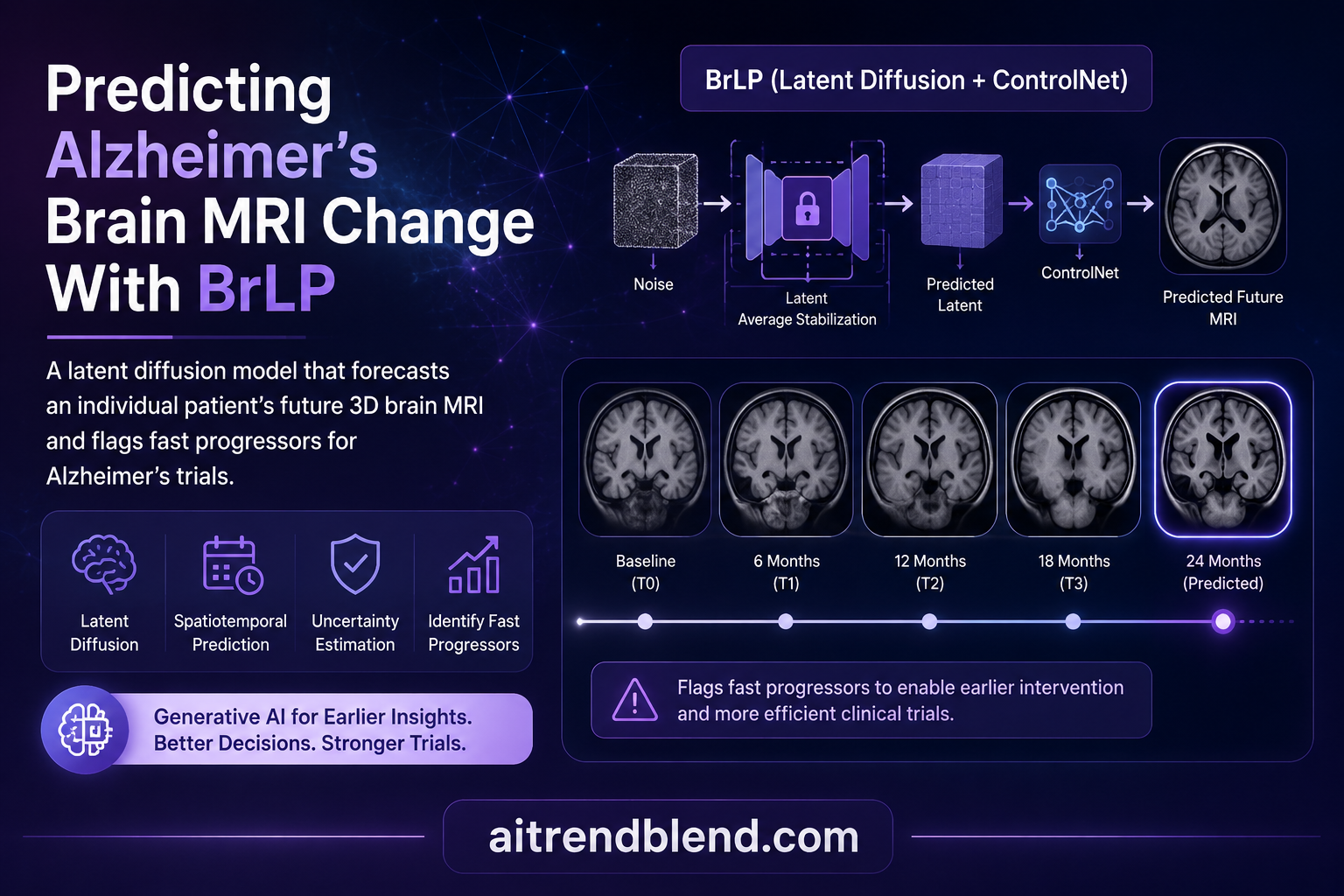
Give a neurologist a brain scan from today and ask what it will look like in five years, and you are asking for something the field has wanted for a long time. Not a population average, not a risk score, but this patient’s brain, aged forward, region by region. A group spanning Catania, London, and Messina built a generative model that attempts exactly that. It takes one 3D brain MRI, a target age, and a few facts about the person, and it paints the future scan, then tells you how much to trust it.
Read this first
This article explains published research. It is not medical advice, diagnosis, or a prognosis for any individual. The model described here predicts imaging patterns in a research setting and has not been validated or approved as a clinical tool. Anyone with questions about Alzheimer’s disease or their own brain health should speak with a qualified clinician.
Key points
- Brain Latent Progression, or BrLP, is a generative model that predicts an individual patient’s future 3D brain MRI from a single baseline scan, a target age, and subject metadata.
- It runs a diffusion model inside a small learned latent space rather than on raw voxels, which is what lets a full 3D scan fit on a consumer grade GPU.
- A ControlNet ties the output to the patient’s own anatomy, and an auxiliary model injects prior knowledge of how brain volumes tend to change with disease.
- A step called Latent Average Stabilization runs the prediction many times and averages the results, which smooths the trajectory over time and doubles as an uncertainty estimate.
- Trained on 11,730 scans from 2,805 people and tested on a separate 2,257 scans from 962 people, BrLP beat prior methods, reaching a structural similarity of about 0.91 against real follow up scans.
- In a retrospective test it flagged fast progressors for a hypothetical trial, finding about 25 percent more of them than random selection, though the whole thing remains a research result rather than a clinical one.
Why forecasting a single brain is so hard
The problem runs deeper than it first appears. Predicting disease progression from images breaks into four demands that fight each other. The first is individualization. Two people the same age with the same diagnosis can follow very different paths, so a model that only learns the average trajectory will be wrong for most individuals. The second is spatiotemporal consistency. If you ask a model for a scan at age seventy, then seventy one, then seventy two, the sequence should evolve smoothly, not jitter around as though it were three unrelated guesses.
The third demand is using longitudinal data well. Hospitals and studies hold repeated scans of the same people over years, and that history carries the signal of how a given brain actually changes, yet many generative approaches ignore it and treat each prediction as a one shot mapping. The fourth is plain engineering. A 3D T1w brain MRI is a large volume, and running a modern diffusion model directly on those voxels is a memory nightmare that pushes researchers toward low resolution volumes that throw away the fine anatomy clinicians care about.
Earlier work tended to solve one demand at the cost of another. Methods built on generative adversarial networks or diffeomorphic warps can reshape an existing scan but cannot invent new structures that were not there, such as the white matter hypointensities that appear in T1w images as disease advances. Methods that shrink the volume to save memory lose detail. BrLP, from Lemuel Puglisi at the University of Catania, Daniel C. Alexander at University College London, and Daniele Ravì at the University of Messina, is an attempt to hold all four demands at once.
The core move, work in latent space
Here is where it gets interesting. Rather than run diffusion on the raw scan, BrLP first trains an autoencoder that compresses each 3D brain MRI into a small latent code. The numbers make the payoff obvious. An input volume of shape 122 by 146 by 122 collapses to a latent of shape 3 by 16 by 20 by 16. That is a reduction of several orders of magnitude in the number of values the generative model has to handle, and it is the reason the whole system fits on ordinary hardware instead of a data center.
Inside that latent space sits a denoising diffusion model. The idea behind diffusion is worth stating plainly because everything else rests on it. During training the model watches clean latents get corrupted by Gaussian noise in many small steps until nothing but noise remains, and it learns to run that process backward, removing a little noise at a time. At generation time you start from pure noise and let the trained network walk it back to a clean latent, which the autoencoder then decodes into a brain. The network is a conditional UNet that predicts the noise added at each step, and it is trained by minimizing the gap between the true noise and its estimate.
Read that as the training target. The term \(\epsilon\) is the real Gaussian noise added to a latent at step \(t\), and \(\epsilon_{\theta}\) is the network’s guess given the noisy latent \(z_t\), the step index, and a set of conditions \(c\). Push that squared error down across the data and the network learns to denoise, which is the same as learning to generate. Those conditions \(c\) are how the model knows whose brain to draw and at what age, and they enter the UNet through a cross attention mechanism in the style of latent diffusion image models.
Keeping the patient in the picture
Conditioning on age and metadata alone is not enough, because it does not tie the output to the specific folds and ventricles of the person in front of you. A latent diffusion model given only covariates can produce a plausible brain of the right age that is not this patient’s brain. BrLP fixes that with a ControlNet, a second network wrapped around the frozen diffusion model whose job is to steer generation toward the subject’s own baseline anatomy. The diffusion weights stay fixed and only the ControlNet is trained, a design that borrows directly from how ControlNet is used to guide image diffusion.
The third ingredient is an auxiliary model that supplies prior knowledge of disease dynamics. Before generating the future scan, this smaller model predicts how the progression related brain volumes, things like hippocampus and lateral ventricle size expressed as a share of total brain volume, should look at the target age. Those predicted volumes become part of the conditioning. The team tried two versions, a linear regression that minimizes a robust loss and a disease course mapping model fitted separately for each cognitive status. This is the piece that lets BrLP fold years of longitudinal knowledge into a single prediction instead of guessing blind.
Latent Average Stabilization, the quiet star
Diffusion generation starts from random noise, so run it twice and you get two slightly different answers. For a single pretty picture that variation is harmless. For a predicted trajectory across many future ages it is a real problem, because the differences show up as irregular jumps from one timepoint to the next, exactly the spatiotemporal inconsistency the method set out to avoid. The team’s answer is a technique they call Latent Average Stabilization, or LAS, and it is disarmingly simple.
LAS runs the whole prediction some number of times, call it \(m\), each starting from a different random seed, and averages the resulting latents before decoding a single brain. The assumption is that each individual run deviates from a stable underlying mean, so averaging many runs converges toward that mean and cancels the seed to seed noise. The same repetition delivers a second gift for free. The spread across the \(m\) runs is a natural measure of how uncertain the model is, both as a single global number and as a full voxel level map computed from the variance of the decoded predictions.
That expression is the voxel uncertainty map. Each of the \(m\) latent predictions \(z_i^{(B)}\) for target age \(B\) is decoded by \(\mathcal{D}\) into a brain, and the map measures how much those decoded brains disagree at every voxel around their mean \(\mu^{(B)}\). Bright spots on the map are places the model is unsure about. That matters more than it might sound, because a prediction that comes with an honest confidence flag is far more usable in medicine than one that does not.
How many runs do you need? The ablation gives a concrete answer. Raising \(m\) from 2 to 64 lowered mean squared error by 7 percent, cut volumetric errors by about 3 percent on average, and improved structural similarity by 0.68 percent, with most gains statistically significant. The cost is linear memory and compute, from 4.6 GB at a single run to 9.6 GB at 64 runs on one GPU. The team settled on 64 as the working value, a straightforward accuracy against resources trade.
What the numbers show
BrLP was trained on a combined internal set of 11,730 T1w scans from 2,805 subjects drawn from three public Alzheimer’s studies, and then tested on an external set of 2,257 scans from 962 subjects it had never seen. That external test is the part worth trusting, because it checks whether the model generalizes rather than memorizes. The comparison against prior methods is stark.
| Method | MSE ↓ | SSIM ↑ | Hippocampus MAE ↓ | Lat. ventricle MAE ↓ |
|---|---|---|---|---|
| DaniNet | 0.016 | 0.623 | 0.030 | 0.257 |
| CounterSynth | 0.010 | 0.824 | 0.030 | 0.310 |
| Latent-SADM | 0.008 | 0.855 | 0.035 | 0.329 |
| BrLP (proposed) | 0.004 | 0.914 | 0.020 | 0.231 |
The numbers tell a clear story here. BrLP roughly halves the mean squared error of the next best method and lifts structural similarity to 0.914, a level where the predicted scans look genuinely close to the real follow ups rather than merely plausible. It also has the lowest error on the regional volumes that clinicians actually track, the hippocampus and the lateral ventricle, both of which change in telling ways as Alzheimer’s advances. On the external test set the picture held, with structural similarity around 0.91 and the same lead over the baselines, which is the reassuring result because it came from data the model never trained on.
The ablation study confirms that each piece earns its place. Starting from a base model, adding LAS improved structural similarity, adding the auxiliary model improved it further, and the full combination of base plus LAS plus auxiliary model was significantly the best across almost every metric, reaching mean squared error of 0.004 and structural similarity of 0.914 against a base of 0.006 and 0.892. Feeding the model the correct cognitive status rather than a wrong one also improved regional accuracy, which is a sign the model is genuinely using the clinical conditioning and not ignoring it.
A predicted scan that arrives with an honest map of where the model is unsure is worth far more to a clinician than a confident picture that hides its own doubt. On why the uncertainty output matters as much as the image
Uncertainty that behaves the way it should
An uncertainty number is only useful if it tracks reality, so the team tested whether it does. Two findings stand out. First, the global uncertainty grows the further into the future the model predicts, which is exactly what should happen, since forecasting fifteen years out is harder than forecasting one. Using a mixed effects model they found uncertainty rose significantly with prediction distance and with its square, both at p < 0.001. Second, higher uncertainty lined up with worse predictions. The squared uncertainty correlated positively with mean squared error and negatively with structural similarity, again at p < 0.001.
Taken plainly, the model is not just confident or not at random. When it is unsure, it tends to be more wrong, and when it is sure, it tends to be more right. That relationship is what makes the uncertainty output actionable rather than decorative. A user could, in principle, discount predictions that come with a high uncertainty flag, or route them for closer human review.
The voxel level maps add a second layer to this. Rather than a single number for the whole brain, they show exactly where the model hesitates, and in the paper those bright regions line up with the places the prediction later turns out to be wrong. Think about what that offers a reader of the scan. Instead of a black box forecast, they get a picture with its own weak spots marked, which is the difference between a tool a clinician might learn to trust and one they would rightly ignore. It also hints at where the method needs work, since the parts of the brain that stay uncertain are the parts future versions should target first.
A concrete use, finding fast progressors
The most tangible application in the paper is about clinical trials. Trials for Alzheimer’s drugs often fail to show an effect not because the drug does nothing but because too many enrolled patients progress too slowly to reveal any benefit within the trial window. That is a Type II error, a missed real effect, and it wastes money and can shelve useful drugs. One fix is to enrich the trial with fast progressors, patients whose disease is moving quickly enough that a treatment effect would show up.
The team ran a retrospective test. Using subjects with two year follow up data from both the internal set of 154 people and the external set of 165 people, they defined ground truth fast progressors by the largest real hippocampal atrophy, then asked BrLP to pick them out in advance. It identified about 25 percent more fast progressors than random selection internally and about 24 percent more externally, performing on par with a dedicated regression model even though it was never trained for this task. That last point is the interesting one. A general purpose generative model of brain aging turned out to be useful for a specific selection job it was not designed for.
The clinical translation gap
This is where the enthusiasm needs a firm hand. Everything above is a research result on curated data, and the distance to a clinic is real. The scans came from established Alzheimer’s research cohorts that were preprocessed with a careful pipeline, bias field correction, skull stripping, registration to a standard space, intensity normalization, and resampling. Real hospital scans arrive on many scanners with many protocols and far messier quality, and nothing in this study shows how BrLP behaves on that kind of input.
There is also a deeper gap between predicting an image and trusting it for a decision. A predicted future scan is a hypothesis about a person’s trajectory, not a diagnosis and not a prognosis a clinician can hand to a patient. The model does not know about treatments the person might start, other illnesses they might develop, or the many non imaging factors that shape a real disease course. The fast progressor result is promising for trial design, an offline research setting with a human in the loop, and that is the right place for it right now. Using a generative forecast to guide the care of an individual would need prospective validation, regulatory review, and a great deal of evidence that does not yet exist. Treat the clinical framing as motivation, not as a result you can act on.
Honest limitations
The authors are candid about the weak spots. The clearest is a smoothing effect in the outputs. Because generation passes through a variational autoencoder, the decoded brains tend to lose some fine grained detail, a known behavior of that kind of compression, and it can blur exactly the small structures that early disease affects. A model that slightly softens the anatomy is a model that may miss subtle change.
The second limitation is a performance gap between healthy and diseased predictions. BrLP does better on cognitively normal subjects than on those with advanced Alzheimer’s, which is the harder and more clinically important case. The team points to disentangling disease from normal aging as the way to close that gap, since the two processes are tangled together in the data and the model does not fully separate them.
A third limitation is structural. The current design assumes a subject’s final cognitive status is known and fixed across the predicted trajectory, rather than modeling the transitions that actually happen, such as a person moving from mild cognitive impairment to Alzheimer’s over the prediction window. Real disease changes stage, and a model that assumes a fixed stage will misjudge anyone who crosses one. The authors name stage transition modeling, richer disease specific covariates, and even genetic data as future directions, which is an honest map of what is missing.
Key takeaway
- Strong benchmark, careful data, real caveats. BrLP is a genuine advance in generative disease modeling, and it is also a research system trained on clean cohorts, softened by its autoencoder, weaker on advanced disease, and untested on the messy scans a hospital produces.
Full implementation in PyTorch
The code below is a compact and runnable reference for the ideas at the heart of BrLP, a conditional latent diffusion model with Latent Average Stabilization and an uncertainty map. It is a teaching implementation rather than the authors’ exact pipeline, using tiny stand in networks and 2D latents so the structure stays readable. It builds a small autoencoder, a noise schedule, a conditional denoiser, the training loss that mirrors the paper’s objective, an auxiliary covariate predictor, the LAS inference loop with a global and voxel level uncertainty estimate, an evaluation routine, and a smoke test on dummy data so you can confirm it runs end to end.
# brlp_reference.py
# A compact, runnable reference for latent diffusion disease progression.
# Educational 2D stand in for the 3D BrLP pipeline, with LAS and uncertainty.

import torch
import torch.nn as nn


class AutoEncoder(nn.Module):
    """Compresses an image into a small latent and decodes it back."""
    def __init__(self, img_ch=1, lat_ch=3):
        super().__init__()
        self.enc = nn.Sequential(
            nn.Conv2d(img_ch, 16, 4, stride=2, padding=1), nn.ReLU(),
            nn.Conv2d(16, lat_ch, 4, stride=2, padding=1))
        self.dec = nn.Sequential(
            nn.ConvTranspose2d(lat_ch, 16, 4, stride=2, padding=1), nn.ReLU(),
            nn.ConvTranspose2d(16, img_ch, 4, stride=2, padding=1))

    def encode(self, x): return self.enc(x)
    def decode(self, z): return self.dec(z)


class NoiseSchedule:
    """Scaled linear beta schedule, the DDPM forward process."""
    def __init__(self, T=1000, b0=1e-4, b1=2e-2):
        self.T = T
        betas = torch.linspace(b0, b1, T)
        self.alpha_bar = torch.cumprod(1.0 - betas, dim=0)

    def add_noise(self, z0, t, eps):
        """Corrupt a clean latent z0 to step t. Returns the noisy latent."""
        ab = self.alpha_bar[t].view(-1, 1, 1, 1)
        return ab.sqrt() * z0 + (1.0 - ab).sqrt() * eps


class CondDenoiser(nn.Module):
    """Predicts the noise in a latent given the step and covariates c."""
    def __init__(self, lat_ch=3, cond_dim=4, ch=32):
        super().__init__()
        self.cond = nn.Linear(cond_dim + 1, ch)   # covariates plus time
        self.body = nn.Sequential(
            nn.Conv2d(lat_ch, ch, 3, padding=1), nn.ReLU(),
            nn.Conv2d(ch, ch, 3, padding=1), nn.ReLU(),
            nn.Conv2d(ch, lat_ch, 3, padding=1))

    def forward(self, z_t, t, c):
        # Inject a simple additive conditioning bias, a stand in for cross attention.
        tc = torch.cat([c, t.float().view(-1, 1) / 1000.0], dim=1)
        bias = self.cond(tc).view(z_t.size(0), -1, 1, 1)
        return self.body(z_t + bias[:, :z_t.size(1)])


def diffusion_loss(denoiser, sched, z0, c):
    """The paper's objective, mean squared error on the predicted noise."""
    b = z0.size(0)
    t = torch.randint(0, sched.T, (b,))
    eps = torch.randn_like(z0)
    z_t = sched.add_noise(z0, t, eps)
    eps_hat = denoiser(z_t, t, c)
    return ((eps - eps_hat) ** 2).mean()


class AuxiliaryModel(nn.Module):
    """Predicts progression covariates at target age from baseline facts."""
    def __init__(self, in_dim=4, out_dim=4):
        super().__init__()
        self.net = nn.Sequential(nn.Linear(in_dim, 16), nn.ReLU(),
                                 nn.Linear(16, out_dim))

    def forward(self, baseline_facts): return self.net(baseline_facts)


def ddim_sample(denoiser, sched, shape, c, steps=50):
    """A short reverse process. Returns one predicted latent."""
    z = torch.randn(shape)
    ts = torch.linspace(sched.T - 1, 0, steps).long()
    for t in ts:
        tb = torch.full((shape[0],), int(t))
        eps_hat = denoiser(z, tb, c)
        ab = sched.alpha_bar[t]
        z0_hat = (z - (1 - ab).sqrt() * eps_hat) / ab.sqrt()
        z = z0_hat + 0.2 * torch.randn_like(z)   # light stochasticity
    return z0_hat


def las_predict(denoiser, sched, ae, shape, c, m=64):
    """
    Latent Average Stabilization.
    Runs the prediction m times, averages the latents for a stable output,
    and returns a decoded brain plus global and voxel level uncertainty.
    """
    lats = torch.stack([ddim_sample(denoiser, sched, shape, c)
                        for _ in range(m)], dim=0)   # (m, B, C, H, W)
    mu = lats.mean(dim=0)
    brain = ae.decode(mu)
    # Voxel uncertainty, variance of decoded predictions around the mean.
    decoded = torch.stack([ae.decode(lats[i]) for i in range(m)], dim=0)
    voxel_unc = decoded.var(dim=0, unbiased=True)
    global_unc = voxel_unc.mean().item()
    return brain, global_unc, voxel_unc


def evaluate(pred, target):
    """Report MSE and a simple global SSIM proxy."""
    mse = ((pred - target) ** 2).mean().item()
    px, py = pred.mean(), target.mean()
    vx, vy = pred.var(), target.var()
    cov = ((pred - px) * (target - py)).mean()
    c1, c2 = 0.01, 0.03
    ssim = ((2 * px * py + c1) * (2 * cov + c2)) / \
           ((px ** 2 + py ** 2 + c1) * (vx + vy + c2))
    return mse, ssim.item()


def smoke_test():
    """End to end check on dummy data. Confirms the pipeline runs."""
    torch.manual_seed(0)
    B, H, W = 4, 64, 64
    imgs = torch.rand(B, 1, H, W)                 # stand in for baseline MRIs
    facts = torch.rand(B, 4)                     # age, sex, diagnosis, volume

    ae = AutoEncoder()
    sched = NoiseSchedule()
    denoiser = CondDenoiser()
    aux = AuxiliaryModel()

    # Quick joint warm up so the parts are not random noise.
    opt = torch.optim.Adam(
        list(ae.parameters()) + list(denoiser.parameters()), lr=1e-3)
    for step in range(50):
        z0 = ae.encode(imgs)
        recon = ae.decode(z0)
        cov = aux(facts)                          # predicted covariates
        loss = ((recon - imgs) ** 2).mean() \
            + diffusion_loss(denoiser, sched, z0.detach(), cov.detach())
        opt.zero_grad(); loss.backward(); opt.step()
    print(f"final training loss {loss.item():.4f}")

    # Predict with LAS using a small m for speed.
    lat_shape = ae.encode(imgs).shape
    cov = aux(facts).detach()
    brain, g_unc, v_unc = las_predict(denoiser, sched, ae, lat_shape, cov, m=8)
    mse, ssim = evaluate(brain, imgs)
    print(f"decoded brain shape {tuple(brain.shape)}")
    print(f"global uncertainty  {g_unc:.5f}")
    print(f"MSE {mse:.4f}  SSIM proxy {ssim:.4f}")


if __name__ == "__main__":
    smoke_test()
The smoke test trains the parts briefly, runs a LAS prediction with a small number of samples for speed, and prints the decoded output shape along with a global uncertainty value and the error metrics. The exact numbers depend on the tiny networks and the short training, so treat this as a structural demonstration rather than a benchmark. To move toward the real system you would replace the stand in autoencoder with a pretrained 3D model, swap the additive conditioning for cross attention, add a ControlNet branch tied to the baseline scan, fit a proper auxiliary model such as disease course mapping, and raise the number of LAS samples toward 64.
Conclusion
The core achievement of this work is a generative model that predicts an individual patient’s future 3D brain MRI with accuracy that clears the prior state of the art, reaching a structural similarity near 0.91 against real follow up scans on data it never trained on. That is not a small step. Forecasting a specific brain, region by region, has resisted easy solutions precisely because individualization, temporal consistency, longitudinal history, and memory all pull against each other, and BrLP holds all four at once.
The conceptual shift underneath the result is worth restating because it travels. Running diffusion in a compact latent space is what makes a full 3D scan tractable on ordinary hardware, and that single choice opens generative disease modeling to hospitals and labs that could never afford a data center. Pair that with a ControlNet that anchors the output to the patient’s own anatomy and an auxiliary model that carries disease knowledge, and you have a system that generates not just a plausible brain but a personalized forecast.
The quiet innovation is Latent Average Stabilization. Averaging many stochastic runs to stabilize a trajectory is a simple idea, and its payoff is double, a smoother and more accurate prediction plus an uncertainty estimate that actually tracks error. In medicine a model that knows when it does not know is worth far more than one that hides its doubt, and the fact that BrLP’s uncertainty rises with prediction distance and lines up with real error is one of the most useful things in the paper.
The honest remaining limitations keep the excitement in proportion. The autoencoder smooths away fine detail, the model is weaker on advanced disease than on healthy aging, it assumes a fixed cognitive status rather than modeling stage transitions, and every result rests on clean research cohorts rather than the messy scans a clinic produces. The fast progressor experiment is promising for trial design, an offline setting with a human in the loop, and that is the right home for it today. None of this undercuts the contribution. It locates it accurately as a strong research advance with a real path forward.
The direction from here is clear enough to name. Disentangling disease from aging, modeling transitions between disease stages, adding richer clinical and even genetic covariates, and testing on real world hospital data would each move the method toward something a care team could use. The code is open, which means others can build on it rather than reinvent it. If those pieces come together, a routine, individualized, honestly uncertain forecast of brain change is a genuinely useful thing to put in front of a clinician, and this work is a serious step toward it.
Frequently asked questions
What does BrLP actually predict?
BrLP predicts an individual patient’s future 3D brain MRI. Given one baseline scan, a target age, and subject metadata such as sex and diagnosis, it generates the scan the model expects at that future age, along with an estimate of how uncertain that prediction is.
Why does BrLP work in a latent space instead of on the raw scan?
A full 3D brain MRI is a very large volume, and running a diffusion model directly on those voxels needs far too much memory. BrLP first compresses each scan into a small latent code with an autoencoder, then runs the diffusion model on that code, which is what lets the whole system run on consumer grade GPUs without discarding anatomical detail.
What is Latent Average Stabilization and why does it matter?
Latent Average Stabilization runs the prediction many times from different random seeds and averages the resulting latents before decoding a single brain. This smooths the predicted trajectory over time and, because the spread across runs reflects disagreement, it also produces a global and voxel level uncertainty estimate for free.
How accurate is BrLP compared to earlier methods?
On both internal and external test sets BrLP outperformed prior methods such as DaniNet, CounterSynth, and Latent-SADM, roughly halving mean squared error and reaching a structural similarity of about 0.91 against real follow up scans, with the lowest error on regional volumes like the hippocampus and lateral ventricle.
Can BrLP be used to diagnose or predict Alzheimer’s in a patient?
No. BrLP is a research model that has not been validated or approved for clinical use. It predicts imaging patterns, not a diagnosis or a personal prognosis, and it was tested on curated research data rather than everyday hospital scans. Any clinical decision requires a qualified professional.
What are the main limitations of BrLP?
The variational autoencoder introduces a smoothing effect that can blur fine detail, the model performs better on healthy aging than on advanced Alzheimer’s, it assumes a fixed cognitive status rather than modeling transitions between disease stages, and all results come from clean research cohorts rather than real world clinical scans.
Puglisi, L., Alexander, D.C., and Ravì, D. BrainLatentProgression, individual based spatiotemporal disease progression on 3D brain MRIs via latent diffusion. Medical Image Analysis, volume 106 (2025), article 103734. University of Catania, University College London, and University of Messina, with data from the Alzheimer’s Disease Neuroimaging Initiative and the Australian Imaging Biomarkers and Lifestyle study. Available at https://doi.org/10.1016/j.media.2025.103734.
This analysis is based on the published paper and an independent evaluation of its claims.
Can you be more specific about the content of your article? After reading it, I still have some doubts. Hope you can help me.