
Key points
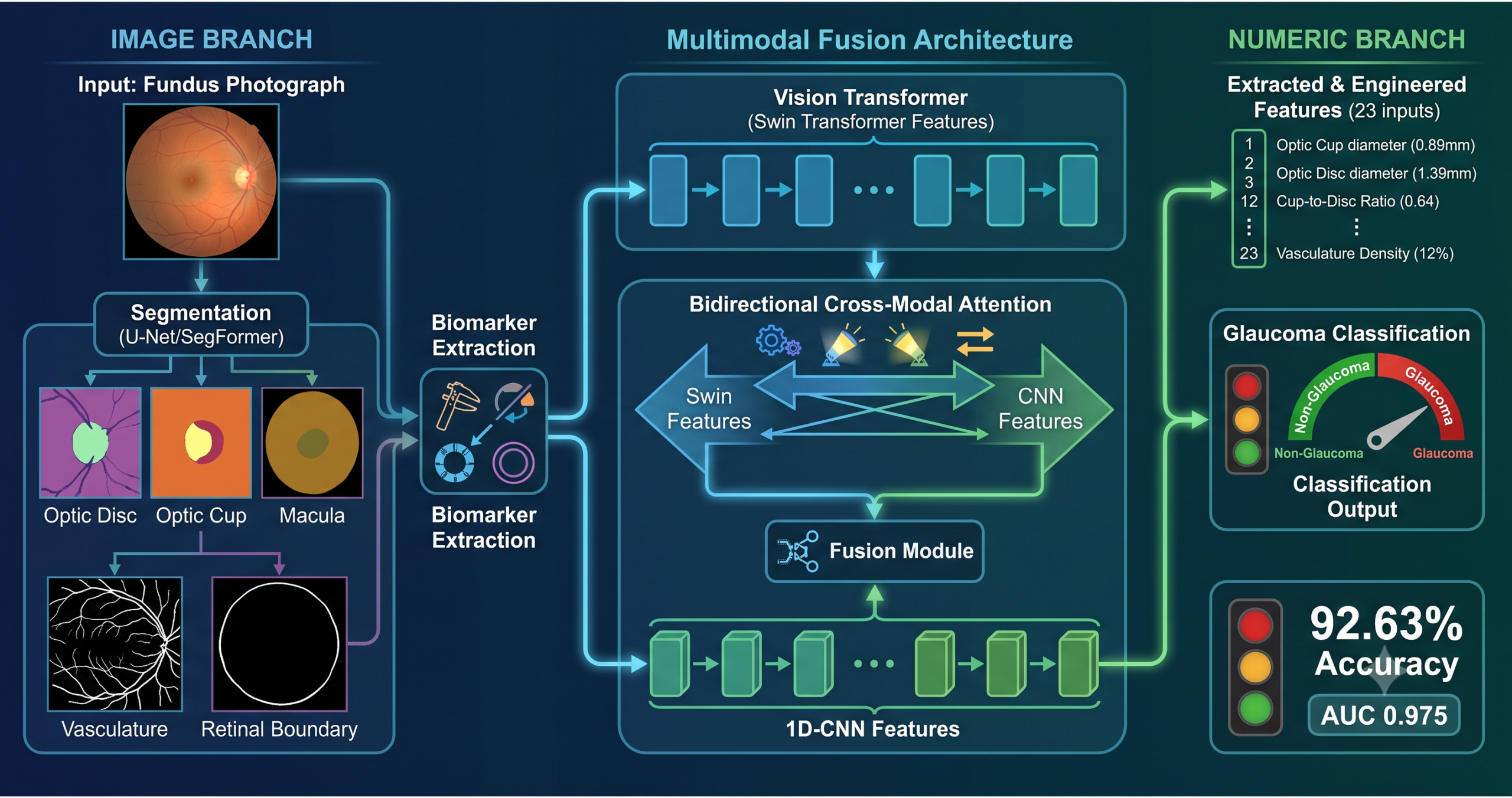
- The pipeline extracts six clinical biomarkers from fundus images using U-Net and SegFormer segmentation models: optic disc diameter, optic cup diameter, retinal vasculature density, macular area, retinal diameter, and from these computes 23 features in total including engineered ratios and geometric measurements.
- The numeric biomarkers alone, processed by a 1D-CNN, achieve 75.51% test accuracy on the SMDG-19 benchmark, which is higher than any single vision transformer in isolation (Swin-b: 66.33%, Swin-V2-b: 72.22%, ViT-b-16: 74.60%). Clinical measurements carry more discriminative signal per feature than raw image representations on their own.
- Bidirectional cross modal attention is used for fusion so that image representations can attend to numeric features and vice versa. This symmetric design produces a measurable shift in both modalities: image features shift by an L2 distance of 13.88 at 64.8 degrees, numeric features by 12.53 at 71.2 degrees, confirming that both modalities are genuinely modified rather than one dominating the other.
- ROAR (RemOve And Retrain) experiments validate that the model relies on meaningful features: masking the top 25% of learned features drops accuracy from 92.63% to 56.35%, and masking 50% drops it to 45.35%.
- The extracted biomarkers closely match clinically established values. The mean extracted cup-to-disc ratio is 0.60 in glaucoma patients and 0.50 in healthy patients, consistent with Crowston et al.’s large population study (N=3,654) which found a median of 0.43 and a 95th percentile of 0.67 in glaucoma.
- The model outperforms both De Souza et al. (88.27%) and Chincholi et al. (90.48%) on the same SMDG-19 benchmark. These comparisons are meaningful; comparisons to methods evaluated on smaller or homogeneous single-source datasets are not directly applicable to this heterogeneous setting.
Why single-modality glaucoma AI falls short
Glaucoma causes progressive damage to the optic nerve and often develops without any early symptoms. This makes early glaucoma detection incredibly vital because existing treatments can only halt or slow down the damage rather than reversing it. Most traditional AI models rely on raw pixels alone. However, this study shows that multimodal glaucoma classification is far more reliable because it pairs raw vision transformer features with exact segmentation derived biomarkers like the cup to disc ratio. This dual approach ensures the model does not miss subtle structural changes that a single modality might overlook.
Fundus photography provides a direct view of the optic disc and cup, and deep learning models trained to classify glaucoma from these images have achieved high accuracy on individual curated datasets. The limitation that this paper addresses is reproducibility across heterogeneous image sources. A model trained on the controlled imaging conditions of one clinic or research dataset tends to lose accuracy when applied to images from different equipment, different acquisition protocols, or different patient populations. The SMDG-19 dataset, assembled from 19 different publicly available glaucoma imaging collections, was specifically designed to evaluate how methods perform under this kind of distribution variability.
The other limitation addressed is interpretability. A model that classifies a fundus image as glaucomatous but cannot explain which features drove that decision is difficult for a clinician to trust or validate. The biomarker extraction pipeline in this paper produces measurements that correspond directly to clinical concepts, optic disc diameter, cup-to-disc ratio, vasculature density, giving both a richer input to the classifier and a transparent accounting of what the model is using.
The segmentation pipeline, four separate models for four anatomical targets
Optic disc and optic cup segmentation with U-Net
The optic disc and cup are the primary anatomical targets for glaucoma assessment. U-Net models are trained separately on each, using 2,805 fundus images with corresponding segmentation masks drawn from SMDG-19 for each task. The optic disc model trains for 30 epochs; the optic cup model trains for 50 epochs because the cup is a smaller region with lower contrast boundaries and greater anatomical variability, requiring more iterations to learn reliable boundary representations. Both use a combined BCE-Dice loss that handles the spatial overlap objective that pixel-wise cross-entropy alone does not optimize well.
| Structure | Model | Test Dice | Test IoU | Test Accuracy |
|---|---|---|---|---|
| Optic disc | U-Net | 0.933 | 0.875 | 0.996 |
| Optic cup | U-Net | 0.829 | 0.709 | 0.998 |
| Retinal vasculature | U-Net | 0.787 | 0.649 | 0.934 |
| Macula | SegFormer | 0.916 | 0.849 | 0.995 |
Once segmentation masks are predicted, contour detection is applied to each mask and a minimum enclosing circle is fitted to the largest detected contour. The diameter of that circle gives the diameter of the structure in pixels. Converting from pixels to millimeters uses a calibration baseline: assuming a retinal diameter of 35mm corresponds to 513.38 pixels in a standard fundus image, each pixel corresponds to approximately 0.068mm. The optic cup Dice of 0.829 is lower than the optic disc at 0.933, which is expected given the cup’s smaller size and less distinct boundaries, and the paper notes this gap honestly rather than treating it as a secondary concern.
Retinal vasculature and macular segmentation
Vasculature density is computed from a U-Net trained on 462 vascular mask images, using a more aggressive augmentation regime that includes Gaussian blur, Gaussian noise, and hue-saturation adjustment to handle the substantial color variability across different fundus camera types. The density value is simply the proportion of image pixels classified as vascular tissue. The macular region is segmented using a custom SegFormer-based architecture that incorporates a Feature Pyramid Network branch and a Squeeze-and-Excitation block before the decoder, producing a semantically rich feature map before refining it through a dedicated refinement module. The 728 macular images were manually annotated because SMDG-19 does not provide macula masks, and the dataset was tripled through augmentation to reach 2,184 training samples.
Retinal diameter extraction without a segmentation model
The retinal boundary itself, rather than any internal structure, is extracted via Canny edge detection followed by contour detection and minimum enclosing circle fitting. This approach does not require a dedicated segmentation model for the retina as a whole. Its accuracy depends on how clearly the retinal boundary is defined in the image and can be affected by noise or poor image quality, which the authors acknowledge as a limitation. The contour detection step between Canny edges and the enclosing circle mitigates some of this fragility by enforcing continuity in the detected boundary.
Feature engineering builds 23 inputs from five raw measurements
Five measurements extracted directly from image processing (retinal diameter, optic disc diameter, optic cup diameter, vasculature density, macular area) are extended through feature engineering into 23 inputs for the 1D-CNN. The engineered features include radii, areas, circumferences, and critically the ratios between structures: optic disc to retina diameter ratio, optic cup to disc diameter ratio, optic cup to disc area ratio, and related variants. These ratio features are clinically meaningful because glaucoma assessment depends on the relationship between structures rather than their absolute sizes, and including them explicitly gives the model access to the same relational information that clinicians use.
The multimodal architecture
The architecture integrates two image branches and one numeric branch. The image branches are Swin-b and Swin-V2-b, selected for complementary strengths. Swin-b provides hierarchical feature extraction through shifted window attention that alternates between non-overlapping local windows and shifted windows, capturing both local and global image context. Swin-V2-b improves on this with residual post-normalization that stabilizes training at higher resolution and larger scale, and is more robust to the varied image quality in SMDG-19. Features from both transformers are concatenated to form the image branch output. The numeric branch is a two-block 1D-CNN where each block consists of a 1D convolutional layer, batch normalization, ReLU activation, and max pooling, progressively building higher-level representations of the input biomarkers.
Before fusion, both branches are linearly projected into a shared embedding space of equal dimensionality (256 dimensions), enabling the attention operations that follow. Self-attention within each modality refines that modality’s own representations. Bidirectional cross modal attention then follows: image features use numeric features as keys and values (letting clinical measurements guide visual attention), and numeric features use image features as keys and values (letting visual context refine the biomarker representations). This symmetric design is motivated by the clinical reality that glaucoma assessment genuinely requires integrating both types of information rather than one leading and the other following.
“The proposed architecture explicitly models both intra-modal and inter-modal dependencies, rather than combining outputs post hoc.” Parikh, Nguyen, Penkova — University of Southern California, Knowledge-Based Systems 2026
What the ablation study reveals
The three-axis ablation study is one of the most informative parts of the paper because it isolates the contribution of each component systematically rather than just comparing the full model to baselines.
Unimodal models in isolation
| Model | Test accuracy | Test recall | Test ROC-AUC |
|---|---|---|---|
| ViT-b-16 | 74.60% | 0.525 | 0.809 |
| 1D-CNN (biomarkers) | 75.51% | 0.701 | 0.822 |
| Swin-V2-b | 72.22% | 0.519 | 0.761 |
| Swin-b | 66.33% | 0.361 | 0.699 |
The 1D-CNN trained only on the 23 extracted biomarkers is the strongest unimodal model. This is the result that most directly validates the claim that clinical biomarkers carry substantial discriminative information. A single transformer operating on the full fundus image without biomarker access cannot match the performance of a simple convolutional network operating on geometrically extracted clinical measurements. DeLong’s test confirms no statistically significant difference between ViT-b-16 and the 1D-CNN (p = 0.475), while all transformer-vs-1D-CNN comparisons involving Swin models are highly significant, suggesting the Swin architectures without biomarkers are weaker on this heterogeneous dataset than a simple biomarker model.
Adding biomarkers to each image model
| Combination | Test accuracy | Test ROC-AUC |
|---|---|---|
| ViT-b-16 + 1D-CNN | 90.93% | 0.961 |
| Swin-b + 1D-CNN | 91.50% | 0.968 |
| Swin-V2-b + 1D-CNN | 91.52% | 0.973 |
Adding biomarkers to any single image model produces a jump of roughly 15 to 25 percentage points in test accuracy. Swin-b goes from 66.33% alone to 91.50% with biomarkers. Swin-V2-b goes from 72.22% to 91.52%. ViT-b-16 goes from 74.60% to 90.93%. The complementary nature of the two modalities is clearest for Swin-b, which is the weakest image-only model but becomes competitive as soon as clinical measurements are added. This finding motivates the decision to drop ViT-b-16 from the final architecture, keeping both Swin models, since ViT-b-16 shows the smallest per-model contribution after combining with biomarkers.
Fusion strategy matters
| Fusion strategy | Test accuracy | Test F1 | Test ROC-AUC |
|---|---|---|---|
| Gated Fusion | 80.95% | 0.778 | 0.867 |
| Feature Concatenation | 91.52% | 0.916 | 0.973 |
| Cross-Modal Attention Fusion | 92.63% | 0.917 | 0.975 |
Gated fusion performs substantially worse than concatenation (80.95% vs 91.52%), suggesting that a learned gate over modality contributions does not work as well as simply concatenating features and letting subsequent layers determine relevance. Cross modal attention improves further over concatenation (92.63% vs 91.52%), with a confidence interval that does not fully overlap with concatenation, supporting the claim that the attention-based fusion is capturing something beyond what simple feature combination provides.
The cross-modal attention shift and what it tells us
The paper goes beyond performance numbers to measure what the cross modal attention blocks actually do to the feature representations. For each modality, the L2 distance between the feature vector before and after cross attention is computed alongside the cosine angle between the two vectors.
The attention score analysis shows that image representations attend most heavily to retina circumference, retina radius, and optic cup circumference in the numeric branch, with additional attention to optic cup and disc diameters, vasculature density, and related ratios. This closely mirrors the features that clinicians prioritize in glaucoma assessment, providing a mechanistic explanation for why the cross modal attention design improves over late fusion: the image branch is learning to query the most clinically relevant numeric signals rather than treating all biomarkers equally.
ROAR experiments confirm genuine feature reliance
The ROAR experiments address a concern that interpretability methods can highlight features that appear important but are not actually used by the model for its predictions. ROAR masks the top k% of features ranked by learned importance and retrains the model on the masked data. If the masked features were genuinely important, performance should drop substantially.
| Features masked | Test accuracy | Test F1 |
|---|---|---|
| None (full model) | 92.63% | 0.917 |
| Top 25% | 56.35% | 0.663 |
| Top 50% | 45.35% | 0.454 |
Masking the top 25% of features drops accuracy from 92.63% to 56.35%, a decline of 36 percentage points. The model retrained without optic disc, optic cup, and retinal geometry information effectively fails on the task, confirming that those features are genuinely driving the classification rather than serving as artifacts of the interpretability method. At 50% masking, the model drops further to 45.35%, which is below chance for a binary classification task, indicating that the remaining features cannot support reliable classification without the lost structural information about vasculature density.
Deployment feasibility
The modular pipeline design separates the computationally lighter segmentation and measurement stages from the transformer-based classification stage, so that the most expensive operations are applied only once per image. The complete pipeline runs in approximately 2.85 seconds per image on a CPU and 0.30 seconds on a GPU, measured on an Intel Xeon at 2.20 GHz and an NVIDIA Tesla P100 respectively, achieving nearly a 10x speedup with GPU acceleration. The multimodal classification step alone takes 1.09 seconds on CPU and 0.12 seconds on GPU. The paper reports that a working deployment was created via a Gradio interface hosted on Hugging Face Spaces, running on default CPU resources, which the authors position as enabling accessible clinical review rather than as a deployment-ready clinical tool.
Clinical limitations
- The framework is trained and evaluated on SMDG-19, which aggregates 19 publicly available research datasets. While this provides heterogeneous imaging conditions, the dataset still consists of retrospective research images rather than prospectively collected clinical screening data. No prospective clinical validation has been conducted, and no regulatory approval of any kind is described.
- The optic cup segmentation achieves a test Dice of 0.829, lower than the optic disc at 0.933. Since cup-to-disc ratio is one of the most important diagnostic indicators, inaccuracies in cup segmentation propagate directly to the most clinically critical biomarker. The paper acknowledges this but does not quantify the downstream effect on biomarker accuracy.
- Retinal diameter extraction relies on Canny edge detection, which can fail when the retinal boundary is not clearly defined, a common occurrence in images of poor quality. The approach may systematically produce less accurate measurements for the image quality ranges where clinical screening is most challenging.
- The 728 macular images were manually annotated because standardized macular masks are not publicly available, introducing annotation subjectivity and limiting the scale of the macular segmentation training data compared to the disc and cup models.
- The model was evaluated on a binary glaucoma-versus-healthy classification task. Glaucoma staging, severity assessment, and distinguishing glaucoma subtypes are separate clinical questions that this framework does not address.
- The dataset has 7,499 non-glaucoma and 4,817 glaucoma images, a class imbalance that may affect recall on the minority class even with the stratified splits used. Calibration to specific clinical false-negative rate requirements would require additional work.
- The deployment demonstration via Gradio and Hugging Face Spaces serves research and review purposes. Clinical deployment of AI tools for disease detection typically requires regulatory review under frameworks such as FDA 510(k) or EU MDR, which have not been pursued for this prototype.
A PyTorch reference implementation
The code below implements the core components of the multimodal architecture described in the paper: the 1D-CNN numeric branch, the bidirectional cross modal attention fusion module, and a simplified multimodal classifier. The biomarker extraction pipeline that feeds the numeric branch requires OpenCV for contour detection and is represented here as a function stub. The full paper is available here.
# multimodal_glaucoma_classifier.py
# Independent educational implementation of the multimodal glaucoma classification
# architecture described in Parikh, Nguyen, Penkova (2026).
# Source paper: Knowledge-Based Systems 349 (2026) 116449.
# DOI: 10.1016/j.knosys.2026.116449
# Not the authors' released code. Written from the method description and figures.

import torch
import torch.nn as nn
import torch.nn.functional as F


# ──────────────────────────────────────────────────────────────────────────────
# Biomarker extraction stub
# In practice this uses OpenCV U-Net and SegFormer predictions.
# Here we return a dictionary of named measurements for demonstration.
# ──────────────────────────────────────────────────────────────────────────────

def extract_biomarkers(disc_mask, cup_mask, vessel_mask, macula_mask, retinal_image):
    """Compute 5 base measurements from segmentation masks.

    disc_mask, cup_mask, vessel_mask, macula_mask: (H, W) binary numpy arrays.
    retinal_image: (H, W) or (H, W, 3) numpy array.
    Returns a dict of floats in pixel units.

    Full pipeline (section 3.2-3.6 of the paper):
    1. Fit minimum enclosing circle to largest contour in disc/cup masks.
    2. Compute vasculature density as vessel_pixels / total_pixels.
    3. Compute macular area as sum of macula mask pixels.
    4. Apply Canny edge detection + contour + enclosing circle for retinal diameter.
    """
    import numpy as np
    # Placeholder: returns fixed values for smoke test
    H, W = retinal_image.shape[:2]
    vessel_pixels = vessel_mask.sum() if vessel_mask is not None else 0
    return {
        "retinal_diameter_px":  513.4,
        "disc_diameter_px":     20.3,
        "cup_diameter_px":      8.9,
        "vasculature_density":  float(vessel_pixels) / max(H * W, 1),
        "macular_area_px2":     4327.0,
    }


def engineer_features(raw: dict) -> list:
    """Compute the full 23-feature vector from 5 raw measurements.

    Derived from Table 6 of the paper: 5 extracted + 18 engineered features
    including radii, areas, circumferences, and inter-structure ratios.
    """
    import math
    rd = raw["retinal_diameter_px"]
    od = raw["disc_diameter_px"]
    cd = raw["cup_diameter_px"]
    vd = raw["vasculature_density"]
    ma = raw["macular_area_px2"]

    rr = rd / 2;   ra = math.pi * rr ** 2;   rc = math.pi * rd
    odr = od / 2;  oda = math.pi * odr ** 2; odc = math.pi * od
    cr = cd / 2;   ca = math.pi * cr ** 2;   cc = math.pi * cd
    mr = math.sqrt(ma / math.pi); md = 2 * mr; mc = math.pi * md

    return [
        rd, od, cd, vd, ma,          # 5 extracted
        rr, ra, rc,                   # retinal geometry
        cr, ca, cc,                   # optic cup geometry
        odr, oda, odc,                # optic disc geometry
        mr, md, mc,                   # macular geometry
        od / max(rd, 1e-6),          # disc-to-retina diameter ratio
        oda / max(ra, 1e-6),         # disc-to-retina area ratio
        cd / max(od, 1e-6),          # cup-to-disc diameter ratio
        ca / max(oda, 1e-6),         # cup-to-disc area ratio
        cd / max(rd, 1e-6),          # cup-to-retina diameter ratio
        ca / max(ra, 1e-6),          # cup-to-retina area ratio
    ]


# ──────────────────────────────────────────────────────────────────────────────
# Numeric branch (1D-CNN, section 3.7)
# Two sequential blocks: Conv1D → BatchNorm → ReLU → MaxPool1D
# ──────────────────────────────────────────────────────────────────────────────

class NumericBranch(nn.Module):
    """1D-CNN that processes the 23-dimensional biomarker feature vector.

    Architecture (section 3.7):
      Block 1: Conv1D(1, ch, k=3) → BN → ReLU → MaxPool1D(2)
      Block 2: Conv1D(ch, ch*2, k=3) → BN → ReLU → MaxPool1D(2)
      Flatten → Linear → BN → ReLU → Linear → output_dim
    """
    def __init__(self, input_dim=23, ch=64, output_dim=256):
        super().__init__()
        self.block1 = nn.Sequential(
            nn.Conv1d(1, ch, kernel_size=3, padding=1),
            nn.BatchNorm1d(ch), nn.ReLU(inplace=True),
            nn.MaxPool1d(2),
        )
        self.block2 = nn.Sequential(
            nn.Conv1d(ch, ch * 2, kernel_size=3, padding=1),
            nn.BatchNorm1d(ch * 2), nn.ReLU(inplace=True),
            nn.MaxPool1d(2),
        )
        flat_dim = ch * 2 * (input_dim // 4)
        self.head = nn.Sequential(
            nn.Flatten(),
            nn.Linear(flat_dim, 256), nn.BatchNorm1d(256), nn.ReLU(inplace=True),
            nn.Linear(256, output_dim),
        )

    def forward(self, x):
        # x: (B, 23) biomarker vector
        x = x.unsqueeze(1)          # (B, 1, 23) for Conv1d
        x = self.block1(x)
        x = self.block2(x)
        return self.head(x)          # (B, output_dim)


# ──────────────────────────────────────────────────────────────────────────────
# Bidirectional cross-modal attention fusion (section 3.7)
# ──────────────────────────────────────────────────────────────────────────────

class CrossModalAttentionFusion(nn.Module):
    """Bidirectional cross-modal attention between image and numeric modalities.

    Steps (section 3.7):
    1. Project both modalities into a shared d_model-dimensional space.
    2. Apply self-attention within each modality.
    3. Apply bidirectional cross-attention:
       - Image queries, numeric keys/values (image attends to biomarkers).
       - Numeric queries, image keys/values (biomarkers attend to image).
    4. Feed-forward network with GELU activation and dropout 0.3.
    5. Concatenate refined representations and pass to classifier head.
    """
    def __init__(self, image_dim, numeric_dim, d_model=256, n_heads=8, dropout=0.3):
        super().__init__()
        self.proj_img = nn.Linear(image_dim, d_model)
        self.proj_num = nn.Linear(numeric_dim, d_model)

        self.self_attn_img = nn.MultiheadAttention(d_model, n_heads, dropout=dropout, batch_first=True)
        self.self_attn_num = nn.MultiheadAttention(d_model, n_heads, dropout=dropout, batch_first=True)
        self.norm_self_img = nn.LayerNorm(d_model)
        self.norm_self_num = nn.LayerNorm(d_model)

        # Image queries attending to numeric keys/values
        self.cross_img2num = nn.MultiheadAttention(d_model, n_heads, dropout=dropout, batch_first=True)
        # Numeric queries attending to image keys/values
        self.cross_num2img = nn.MultiheadAttention(d_model, n_heads, dropout=dropout, batch_first=True)
        self.norm_cross_img = nn.LayerNorm(d_model)
        self.norm_cross_num = nn.LayerNorm(d_model)

        self.ffn = nn.Sequential(
            nn.Linear(d_model * 2, d_model * 2),
            nn.GELU(),
            nn.Dropout(dropout),
            nn.Linear(d_model * 2, d_model),
        )
        self.norm_ffn = nn.LayerNorm(d_model)

    def forward(self, img_feat, num_feat):
        # img_feat: (B, image_dim), num_feat: (B, numeric_dim)
        img = self.proj_img(img_feat).unsqueeze(1)   # (B, 1, d_model)
        num = self.proj_num(num_feat).unsqueeze(1)   # (B, 1, d_model)

        # Self-attention within each modality
        img_sa, _ = self.self_attn_img(img, img, img)
        img = self.norm_self_img(img + img_sa)
        num_sa, _ = self.self_attn_num(num, num, num)
        num = self.norm_self_num(num + num_sa)

        # Bidirectional cross-attention
        img_ca, _ = self.cross_img2num(img, num, num)  # img queries numeric
        img_out = self.norm_cross_img(img + img_ca)
        num_ca, _ = self.cross_num2img(num, img, img)  # numeric queries image
        num_out = self.norm_cross_num(num + num_ca)

        # Fuse and feed-forward
        fused = torch.cat([img_out.squeeze(1), num_out.squeeze(1)], dim=-1)  # (B, 2*d_model)
        out = self.norm_ffn(self.ffn(fused) + fused[:, :fused.shape[-1]//2])  # residual on first half
        return out  # (B, d_model)


# ──────────────────────────────────────────────────────────────────────────────
# Multimodal classifier (simplified, using a mock image encoder)
# In real deployment replace MockImageEncoder with Swin-b + Swin-V2-b concat
# ──────────────────────────────────────────────────────────────────────────────

class MockImageEncoder(nn.Module):
    """Placeholder for Swin-b + Swin-V2-b concatenated image branch."""
    def __init__(self, out_dim=1024):
        super().__init__()
        self.conv = nn.Sequential(
            nn.AdaptiveAvgPool2d((4, 4)),
            nn.Flatten(),
        )
        self.proj = nn.LazyLinear(out_dim)

    def forward(self, x):  # x: (B, 3, 224, 224)
        x = self.conv(x)
        return self.proj(x)


class MultimodalGlaucomaClassifier(nn.Module):
    def __init__(self, n_biomarkers=23, d_model=256, n_classes=2, dropout=0.3):
        super().__init__()
        self.image_encoder = MockImageEncoder(out_dim=1024)
        self.numeric_branch = NumericBranch(input_dim=n_biomarkers, output_dim=d_model)
        self.fusion = CrossModalAttentionFusion(
            image_dim=1024, numeric_dim=d_model, d_model=d_model
        )
        self.classifier = nn.Sequential(
            nn.Linear(d_model, d_model // 2), nn.GELU(), nn.Dropout(dropout),
            nn.Linear(d_model // 2, n_classes),
        )

    def forward(self, image, biomarkers):
        img_feat = self.image_encoder(image)          # (B, 1024)
        num_feat = self.numeric_branch(biomarkers)    # (B, 256)
        fused = self.fusion(img_feat, num_feat)       # (B, 256)
        return self.classifier(fused)                # (B, 2)


# ──────────────────────────────────────────────────────────────────────────────
# Smoke test
# ──────────────────────────────────────────────────────────────────────────────

def smoke_test():
    device = torch.device("cpu")
    model = MultimodalGlaucomaClassifier(n_biomarkers=23, d_model=256).to(device)
    B = 4
    images = torch.randn(B, 3, 224, 224, device=device)
    biomarkers = torch.randn(B, 23, device=device)

    model.train()
    optimizer = torch.optim.Adam(model.parameters(), lr=1e-4, weight_decay=1e-5)
    labels = torch.randint(0, 2, (B,), device=device)

    optimizer.zero_grad()
    logits = model(images, biomarkers)
    loss = F.cross_entropy(logits, labels)
    loss.backward()
    optimizer.step()

    print(f"Smoke test passed.")
    print(f"  Input: images {tuple(images.shape)}, biomarkers {tuple(biomarkers.shape)}")
    print(f"  Output logits: {tuple(logits.shape)}")
    print(f"  Loss: {loss.item():.4f}")
    print(f"  Predicted classes: {logits.argmax(dim=1).tolist()}")

    # Verify feature engineering
    import numpy as np
    raw = extract_biomarkers(None, None, np.zeros((128, 128)), None, np.zeros((128, 128)))
    features = engineer_features(raw)
    assert len(features) == 23, f"Expected 23 features, got {len(features)}"
    print(f"  Feature vector length: {len(features)} (correct)")
    print(f"  Cup-to-disc diameter ratio: {features[19]:.4f}")


if __name__ == "__main__":
    smoke_test()
Conclusion
The paper makes a case that deserves careful reading: segmentation-derived clinical biomarkers, processed by a simple 1D-CNN, outperform vision transformers operating directly on fundus images when those transformers are used in isolation. This is not a minor result. It suggests that the geometric information encoded in the relationship between the optic disc, the optic cup, and the surrounding retinal structures is highly compressible into a small number of well-chosen features, and that deep learning models processing raw pixels must work substantially harder to recover the same discriminative signal that clinicians extract through straightforward measurement.
The ROAR experiments provide the strongest evidence that the pipeline is genuinely learning clinical structure rather than fitting to dataset artifacts. A drop from 92.63% to 56.35% accuracy when the top quartile of features is removed is not consistent with a model that has learned to classify on incidental image properties. The features being masked are real, they are the optic disc region, the cup geometry, and related biomarkers, and the model cannot function without them.
The cross modal attention analysis adds a mechanistic dimension to what is otherwise a benchmark-focused paper. Showing that image representations shift by 64.8 degrees and numeric representations shift by 71.2 degrees after bidirectional cross attention, and that the features most strongly attended to are precisely the retinal geometry measurements clinicians use in practice, bridges the gap between a machine learning result and a clinically interpretable system. It is the kind of analysis that should accompany any clinical AI paper that claims interpretability rather than simply deploying Grad-CAM visualizations and calling the result interpretable.
The honest limitations section is worth noting. The paper does not claim clinical deployment readiness, does not assert that 92.63% accuracy on a research benchmark is sufficient for clinical use, and explicitly identifies the cup segmentation accuracy as a gap that could affect biomarker quality. The deployment demonstration via a Gradio interface is presented as a research validation tool rather than as evidence of clinical applicability. These are the right epistemic postures for a research paper in this domain, and they make the findings more credible rather than less.
The path from this research prototype to a clinically useful tool runs through prospective validation studies, regulatory review, and the kind of comparative clinical evaluation against ophthalmologist judgment that a benchmark comparison cannot substitute for. The algorithmic foundations demonstrated here, particularly the biomarker extraction pipeline whose outputs match known clinical reference values, and the ROAR-validated reliance on anatomically meaningful features, provide a solid basis for that next stage of work.
Frequently asked questions
What clinical glaucoma biomarkers does the pipeline extract
The pipeline extracts optic disc diameter, optic cup diameter, retinal vasculature density, macular area, and retinal diameter using a combination of U-Net segmentation, SegFormer segmentation, and Canny edge detection with minimum enclosing circle fitting. From these five direct measurements, 18 additional features are engineered including radii, areas, circumferences, and inter-structure ratios such as the cup-to-disc diameter ratio, yielding a total of 23 features for the numeric branch.
Why do the numeric biomarkers outperform vision transformers in isolation
The 1D-CNN trained on extracted biomarkers achieves 75.51% test accuracy, higher than Swin-b at 66.33%, Swin-V2-b at 72.22%, and ViT-b-16 at 74.60%. The explanation is that the 23 engineered features encode the geometric relationships between anatomical structures that clinicians use for diagnosis, particularly the cup-to-disc ratio. Vision transformers processing raw fundus pixels must implicitly recover these relationships from pixel-level patterns across a heterogeneous 19-source dataset, which is substantially harder than having those relationships provided explicitly.
What is bidirectional cross-modal attention and why is it used
Bidirectional cross-modal attention allows both modalities to actively query each other’s representations. Image features use clinical biomarkers as keys and values, letting anatomical measurements guide attention toward visually relevant regions. Clinical measurements use image features as keys and values, letting visual context refine the biomarker representations. This symmetric design is motivated by the clinical reality that glaucoma assessment requires both structural visual information and quantitative measurements together rather than one directing the other in a single direction.
What do the ROAR experiments demonstrate
ROAR (RemOve And Retrain) experiments confirm that the model genuinely relies on the learned features rather than learning to classify on incidental or spurious properties. Masking the top 25% of features by importance and retraining drops accuracy from 92.63% to 56.35%, and masking 50% drops it to 45.35%. A model that had learned on irrelevant features would not show this kind of catastrophic degradation when the important features are removed.
Is this system ready for clinical use
No. The system is a research prototype evaluated on retrospective publicly available datasets. No prospective clinical validation has been conducted, and no regulatory approval has been sought. The accuracy reported (92.63% on SMDG-19) reflects performance in a research benchmark setting with stratified splits, not in a prospective clinical screening context. Anyone concerned about glaucoma should consult a qualified ophthalmologist for proper evaluation and diagnosis.
Read the complete segmentation pipeline, all ablation results, and full interpretability analysis in the source paper.