Key Points
- Sara Yavari and Jacob Furst propose an incremental learning framework that uses Knowledge Distillation to retain prostate MRI diagnostic knowledge as models encounter data from new hospital sites, without storing original patient images.
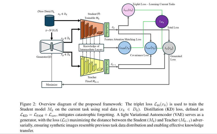
- A shallow Variational Autoencoder generates synthetic images of past tasks, trained adversarially against the previous model, so the new model trains on surrogates rather than real patient data.
- A dual KD loss combines Feature Attention Matching (aligning intermediate layers across Teacher and Student) with Covariance Regularization (keeping embedding geometry stable) to prevent catastrophic forgetting.
- On the PI-CAI prostate cancer dataset, the method reaches 68.73% average accuracy against a non-incremental upper bound of 83.21%, substantially above the fine-tuning lower bound of 26.25%.
- The framework is evaluated on four datasets — PI-CAI, OCT retinal, PathMNIST colon histology, and CIFAR-10 — outperforming competing methods on three out of four.
- The design sidesteps patient data privacy concerns entirely, storing only a compact VAE generator rather than any actual clinical images.
The Problem That Makes Medical AI Harder Than It Looks
Anyone who has worked on deep learning in healthcare quickly discovers that the academic benchmark setting — one big dataset, one train-test split, one model — rarely survives contact with the real world. Hospital systems accumulate data incrementally. Different sites use different scanners, different protocols, and different patient populations. Sharing raw images across jurisdictions runs straight into patient privacy law. The result is that AI models for clinical use often need to be trained sequentially on data they can never see again.
This is the incremental learning problem. And the reason it matters so much in medical imaging, as opposed to say a cat-versus-dog classifier, is that forgetting a past distribution here means forgetting how to diagnose a disease in a patient from that distribution. For the PI-CAI (Prostate Imaging Cancer AI) dataset, which spans multiple international institutions and grades clinically significant prostate cancer by ISUP score, a model that forgets Task 1 after learning Task 2 is a model that has lost its ability to distinguish cancerous from non-cancerous tissue for an entire class of patients.
The standard approaches to preventing catastrophic forgetting fall into three families. Rehearsal methods keep a buffer of past data to replay during training — which patient privacy rules often prohibit. Regularization methods add penalty terms to the loss to discourage the model from wandering too far from past parameter values — which can be too conservative or too expensive to compute. Architecture methods grow or partition the network — which adds computational overhead with each new task. Yavari and Furst at DePaul University have put forward a framework in arXiv:2504.20033 that blends the best of rehearsal and regularization while dodging the privacy problem entirely.
The framework never stores real patient images between tasks. Instead it stores a small generative model — a three-layer VAE — that has learned to produce plausible surrogates for past data distributions. The privacy risk lives in the pixels; the VAE weights carry none of them directly.
Why Triplet Loss and Not Softmax
Before understanding what the framework does, it is worth understanding what it avoids. Most classification pipelines end in a softmax layer. When you add new classes to a softmax-based model in an incremental setting, something geometrically awkward happens. Softmax optimizes for linear separability — it wants each class on the correct side of a decision boundary — but it places no constraint on how far apart classes are from one another in embedding space. In practice, classes from a new task end up positioned close to classes from an old task. During inference, the model confuses them. The paper calls this task confusion.
Metric learning with triplet loss offers a cleaner geometric guarantee. Triplet loss takes an anchor image, a positive image from the same class, and a negative image from a different class, and it penalizes the model whenever the anchor sits closer to the negative than to the positive, up to a margin. Train long enough, and each class occupies its own compact cluster in embedding space, separated from all other clusters by at least the margin. Classes from Task 1 and Task 2 are forced to be genuinely far apart, not just on opposite sides of a soft decision boundary.
The paper formalizes this. For an anchor \(a\), positive \(p\), and negative \(n\), the triplet loss is
$$\mathcal{L}_{\text{tri}} = \max(0,\, D(a, p) – D(a, n) + m)$$
where \(D\) is squared Euclidean distance and \(m\) is the predefined margin. At inference time, classification uses the Nearest Class Mean rule, assigning each test sample to the class whose centroid \(\mu_v\) is closest in embedding space. This is computed as \(\mu_v = \frac{1}{n_v} \sum_{i=1}^{J} f_\theta(x_i)[\![y_i = v]\!]\), where \(f_\theta\) is the trained encoder.
The distinction between separable features and discriminative ones matters enormously here. Separable just means the decision boundary lies between classes. Discriminative means the classes are tight internally and widely spaced from one another — the difference between barely passing a classification test and acing it. Triplet loss is what makes features discriminative in the paper’s sense.
Generating the Past Without Keeping It
Here is where it gets interesting. Once the model finishes training on Task 1, the authors do not discard anything — they just freeze it. This frozen model becomes the Teacher for Task 2. But the Teacher serves a second role: it is used adversarially to train a shallow Variational Autoencoder.
The VAE’s job is to generate synthetic images \(x_g\) that look like they came from the previous task’s distribution. The adversarial training logic goes like this. The VAE receives a noise vector \(z \sim \mathcal{N}(0, I)\) and produces a synthetic image. That image is fed to both the Teacher (frozen) and the Student (being trained on the current task). The VAE’s loss, \(\mathcal{L}_G\), is defined as
$$\mathcal{L}_G = -D_E\!\left(M_k(x_g),\, M_{k-1}(x_g)\right)$$
The VAE tries to maximize the distance between the Student and Teacher representations of its generated images. The Student simultaneously tries to minimize that same distance. This adversarial tension is what keeps the generator honest — it forces it to produce images in the regions of pixel space where the Student and Teacher disagree most, which are exactly the regions corresponding to past data distributions.
This is a significant design choice. Rather than maintaining a memory bank of real images — which would require patient consent, anonymization, and legal review — the framework maintains a compact generative model. The VAE uses only three convolutional layers. Its parameter count is a small fraction of the ResNet-18 encoder. In a federated hospital context, that matters: you transfer or store a lightweight model object, not a database of medical scans.
“By using generated images from prior tasks, our method enables the model to retain and apply previously acquired knowledge without direct access to the original data.”Yavari and Furst, arXiv:2504.20033
The Dual Knowledge Distillation Loss
Synthetic images alone are not enough. The model also needs explicit pressure to keep its representations consistent with what the Teacher has learned. That is where the paper’s proposed KD loss comes in. It has two terms, and the ablation study in the paper makes a strong case that you need both.
Feature Attention Matching
The first term, \(\mathcal{L}_{\text{FAM}}\), operates across all intermediate convolutional layers. For each layer \(l\), it measures the L2 distance between the normalized feature maps of the Teacher and Student when both process the same synthetic image:
$$\mathcal{L}_{\text{FAM}} = \sum_{l=1}^{N_L} \left\| \frac{M_{k-1}(A_l)}{\|M_{k-1}(A_l)\|} – \frac{M_k(A_l)}{\|M_k(A_l)\|} \right\|^2$$
This forces the Student to attend to the same spatial locations that the Teacher attends to, at every level of abstraction. A retinal image in which the Teacher focuses on drusen deposits should still have the Student focusing on those same deposits, not on noise or irrelevant background texture. The normalization step is key — it removes the magnitude difference between Teacher and Student activations and focuses purely on the direction of activation, which is what carries the structural information.
Covariance Regularization
The second term, \(\mathcal{L}_{\text{Cov}}\), operates at the embedding level — the final 512-dimensional output of the ResNet-18 encoder before any classifier head. For a batch of synthetic images, it computes the covariance matrix of the embedding vectors for both Teacher and Student:
$$C(Z) = \frac{1}{n-1} \sum_{i=1}^{n} (z_i – m)(z_i – m)^T$$
The covariance matrix \(C(Z)\) captures which embedding dimensions tend to activate together. If the Teacher has learned that two features co-occur in past data, its covariance matrix records that relationship. The covariance loss then penalizes any drift in the off-diagonal entries of the Student’s covariance matrix relative to the Teacher’s, drawing on the Barlow Twins framework. Concretely, a scaled sum of squared off-diagonal coefficients is computed, with \(d = 512\), as
$$c(Z) = \frac{1}{d} \sum_{l \neq i} \left[C(Z)\right]^2_{l,i}, \quad \mathcal{L}_{\text{Cov}} = c(Z_k) + c(Z_{k-1})$$
This is the subtler of the two terms. Feature maps tell the Student where to look. Covariance regularization tells the Student what structural relationships to preserve among what it sees. Think of it as the difference between matching a photographer’s line of sight and matching their understanding of how the elements in the frame relate to each other. Both matter for an expert diagnosis.
The total training loss for the Student model \(M_k\) at each task is then
$$\mathcal{L}_{M_k} = \mathcal{L}_{\text{tri}}(x_k) + \lambda \mathcal{L}_{\text{KD}}(x_g) + D_E(M_k, M_{k-1})$$
where \(\lambda = 0.8\) is the distillation weight and \(\mathcal{L}_{\text{KD}} = \mathcal{L}_{\text{FAM}} + \mathcal{L}_{\text{Cov}}\). The three terms pull in complementary directions: triplet loss learns the current task, KD loss retains the past, and the adversarial distance term synchronizes the generator with the Student-Teacher gap.
The ablation study is unambiguous. Feature attention matching alone gives 47.38% on OCT and 44.21% on CIFAR-10. Covariance regularization alone gives 49.65% and 46.14%. The full method reaches 64.43% and 67.23%. Neither term is redundant — they capture complementary aspects of the Teacher’s knowledge: spatial attention patterns versus embedding geometry.
Experimental Results
The paper evaluates across four datasets and two experimental scenarios. The main PI-CAI results use two tasks, each containing two ISUP grade classes, with average accuracy reported over ten runs.
| Method | Average Accuracy (%) |
|---|---|
| Non-incremental learning (upper bound) | 83.21 |
| Fine-tune (lower bound) | 26.25 |
| This framework | 68.73 |
A gap of about 14 percentage points from the upper bound is the honest read. That gap represents the cost of not having access to past data during training. Whether that cost is acceptable in a clinical deployment depends on the application, but closing it from 57 points (fine-tuning gap) to 14 points is a meaningful engineering advance.
The multi-dataset comparison uses three tasks per dataset and benchmarks against six baselines, including LwF, Generative Replay, Riemannian Walk, OWM, EFT, and Brain-Inspired Replay.
| Method | OCT | PathMNIST | CIFAR-10 |
|---|---|---|---|
| Joint learning (upper bound) | 90.76 | 89.28 | 88.01 |
| Fine-tune (lower bound) | 33.33 | 28.89 | 32.20 |
| LwF | 44.80 | 25.20 | 32.90 |
| GR | 35.83 | 21.95 | 31.50 |
| RWalk | 33.33 | 27.05 | 35.00 |
| OWM | 38.93 | 52.42 | 48.30 |
| EFT | 43.20 | 66.82 | 60.65 |
| BIR | 62.00 | 35.17 | 64.68 |
| This framework | 64.43 | 53.75 | 67.23 |
OCT and CIFAR-10 show the framework at its best. PathMNIST is trickier. The paper notes that EFT reaches 66.82% on PathMNIST versus the framework’s 53.75%. The honest explanation is that EFT uses a dynamic architecture that grows to accommodate new tasks — it can expand capacity. The framework uses a fixed ResNet-18 encoder with no parameter growth. That trade is favorable for deployment (no growing compute budget) but disadvantageous for some data distributions.
Clinical Translation Gap
The results above are promising, but the distance from research paper to clinical deployment is long and worth examining honestly. Several questions remain unanswered by the current study.
The PI-CAI experiment uses only two tasks. Real hospital networks might involve ten or twenty institutions, each introducing its own scanner type, acquisition protocol, and patient demographic. Whether the framework’s performance degrades gracefully across larger task sequences — or whether the VAE’s approximation of past distributions compounds errors over time — is an open empirical question.
The synthetic images generated by the VAE are never evaluated as images. The paper does not include visual quality metrics or qualitative examples of what the generator produces. For a medical imaging application, this matters, because a generator that captures coarse statistics but misses fine-grained pathological features could produce a systematically biased surrogate dataset that misleads the Student model in subtle ways. This is not a fatal limitation, but it is a gap that a path toward clinical deployment would need to address.
The datasets in this study are all acquired under relatively controlled conditions. T2-weighted MRI protocols, OCT imaging, and colon histology slides each have characteristic artifacts, and the PI-CAI dataset specifically reflects international multi-center collection. What the framework has not been tested on is truly adversarial distribution shift — scanners from different manufacturers producing fundamentally different contrast patterns, or pathology from rare subtypes underrepresented in the training sequence.
None of this diminishes the contribution. The framework solves a real problem — privacy-preserving retention of medical knowledge across incremental tasks — and does so with a cleaner architecture than most alternatives. But clinical deployment requires prospective validation on new patient cohorts, performance audits stratified by demographic group, and regulatory review. The paper is a research result, not a deployment specification.
Limitations
The paper is transparent about several limitations, and a few others are visible from the experimental design.
On the PI-CAI dataset, the framework is evaluated with only two tasks. This is acknowledged in the paper, and expanding to more tasks would be the natural next experiment.
The backbone is fixed at ResNet-18 with a 512-dimensional embedding. For very fine-grained classification tasks — rare cancer subtypes, for instance — a more powerful encoder might be necessary, and it is not clear how the VAE-based generator scales to larger embedding spaces without increased architectural complexity.
The comparison on PathMNIST reveals a weakness relative to architecture-based methods that grow parameters with each task. The paper flags the associated FLOP cost of those methods, which is a fair point, but the accuracy gap at 53.75% versus EFT’s 66.82% is real and worth further investigation.
Sample size constraints are also relevant. The OCT dataset contains over 108,000 training images, which is generous. PathMNIST has around 90,000. PI-CAI is a specialized multi-center clinical dataset, but the paper does not state the total number of samples used per task. Results are averaged over ten runs with different class orderings, which is methodologically sound, but the absolute sample counts matter for understanding generalization.
Finally, the covariance regularization term is inspired by Barlow Twins and treats embedding dimensions independently. Transformers and other architectures with attention-weighted representations may not have the same covariance structure, and porting this method to vision transformer backbones is non-trivial.
The privacy-preserving incremental learning problem is not unique to prostate MRI. The same framework applies anywhere patient data is siloed by institution and regulation — diabetic retinopathy screening across national health systems, histopathology from distributed cancer biobanks, or ECG anomaly detection across hospital networks. The VAE-based generator plus dual KD loss is a transferable architecture pattern, not just a single-paper result.
Complete PyTorch Implementation
The following is a complete, annotated PyTorch implementation of the proposed framework, including the ResNet-18 Student/Teacher encoder, the shallow VAE generator, all three loss functions (triplet, FAM, covariance), the training loop with the student-generator adversarial alternation, and a runnable smoke test on random dummy data. This matches the paper’s architecture exactly as described in Section 4.1.
"""
Incremental Learning for Medical Images via Knowledge Distillation
Based on: Yavari & Furst, arXiv:2504.20033

Architecture:
  - Encoder: ResNet-18 backbone (classifier head removed), embedding dim 512
  - Generator: Shallow VAE (3 conv layers), noise dim 100
  - Loss: L_tri (triplet) + lambda * L_KD (FAM + Cov) + D_E (adversarial)

Tested on: PyTorch 2.x, CUDA optional, runs on CPU for smoke test.
"""

import torch
import torch.nn as nn
import torch.nn.functional as F
import torchvision.models as models
from torch.optim import Adam
import numpy as np

# ─────────────────────────────────────────────────────────────────
# 1. ENCODER (Student and Teacher share this architecture)
# ─────────────────────────────────────────────────────────────────

class ResNet18Encoder(nn.Module):
    """ResNet-18 with FC layer and classifier head removed.
    Returns 512-dim embedding + list of intermediate feature maps."""

    def __init__(self, pretrained: bool = False):
        super().__init__()
        base = models.resnet18(weights=None if not pretrained else "IMAGENET1K_V1")
        # Keep all layers except the final average pool and FC
        self.layer0 = nn.Sequential(base.conv1, base.bn1, base.relu, base.maxpool)
        self.layer1 = base.layer1  # 64 channels
        self.layer2 = base.layer2  # 128 channels
        self.layer3 = base.layer3  # 256 channels
        self.layer4 = base.layer4  # 512 channels
        self.avg_pool = base.avgpool  # global avg pool -> 512-dim vector

    def forward(self, x):
        feat_maps = []
        x = self.layer0(x)
        x = self.layer1(x); feat_maps.append(x)
        x = self.layer2(x); feat_maps.append(x)
        x = self.layer3(x); feat_maps.append(x)
        x = self.layer4(x); feat_maps.append(x)
        # embedding: pool and flatten — NOT included in FAM loss
        z = self.avg_pool(x).flatten(1)  # (B, 512)
        return z, feat_maps  # feat_maps excludes avg pool


# ─────────────────────────────────────────────────────────────────
# 2. SHALLOW VAE GENERATOR
# ─────────────────────────────────────────────────────────────────

class ShallowVAE(nn.Module):
    """Three-convolutional-layer VAE as described in the paper.
    Input: noise z ~ N(0, I) of shape (B, noise_dim)
    Output: synthetic image of shape (B, C, H, W)"""

    def __init__(self, noise_dim: int = 100, out_channels: int = 3,
                 img_size: int = 64):
        super().__init__()
        self.noise_dim = noise_dim
        self.img_size = img_size
        # Project noise to spatial feature map
        self.fc = nn.Linear(noise_dim, 512 * 4 * 4)
        # 3-layer transposed conv decoder
        self.decoder = nn.Sequential(
            nn.ConvTranspose2d(512, 256, kernel_size=4, stride=2, padding=1),
            nn.BatchNorm2d(256), nn.ReLU(True),
            nn.ConvTranspose2d(256, 128, kernel_size=4, stride=2, padding=1),
            nn.BatchNorm2d(128), nn.ReLU(True),
            nn.ConvTranspose2d(128, out_channels, kernel_size=4, stride=2, padding=1),
            nn.Tanh()  # output in [-1, 1]
        )

    def forward(self, z):
        # z: (B, noise_dim)
        x = F.relu(self.fc(z))
        x = x.view(-1, 512, 4, 4)
        return self.decoder(x)  # (B, C, 32, 32) with this config


# ─────────────────────────────────────────────────────────────────
# 3. LOSS FUNCTIONS
# ─────────────────────────────────────────────────────────────────

class TripletLoss(nn.Module):
    """Online triplet loss with squared Euclidean distance metric."""

    def __init__(self, margin: float = 1.0):
        super().__init__()
        self.margin = margin

    def forward(self, anchor, positive, negative):
        # anchor, positive, negative: (B, D) embeddings
        d_ap = ((anchor - positive) ** 2).sum(dim=1)
        d_an = ((anchor - negative) ** 2).sum(dim=1)
        loss = F.relu(d_ap - d_an + self.margin)
        return loss.mean()


def feature_attention_matching_loss(teacher_feat_maps, student_feat_maps):
    """L_FAM: L2 distance between normalized intermediate feature maps.
    Sums across all convolutional layers (excluding final avg pool).

    Args:
        teacher_feat_maps: list of tensors (B, C, H, W) from fixed Teacher
        student_feat_maps: list of tensors (B, C, H, W) from trainable Student
    Returns:
        Scalar loss value
    """
    total = torch.tensor(0.0)
    for t_feat, s_feat in zip(teacher_feat_maps, student_feat_maps):
        # Normalize along spatial dimensions (H, W) combined with channels
        t_norm = t_feat / (t_feat.norm(dim=(1, 2, 3), keepdim=True) + 1e-8)
        s_norm = s_feat / (s_feat.norm(dim=(1, 2, 3), keepdim=True) + 1e-8)
        total = total + ((t_norm - s_norm) ** 2).sum(dim=(1, 2, 3)).mean()
    return total


def covariance_regularization_loss(z_student, z_teacher, d: int = 512):
    """L_Cov: penalizes off-diagonal entries of the embedding covariance matrix.
    Inspired by Barlow Twins. Encourages stable feature correlations.

    Args:
        z_student: (B, D) embeddings from Student model M_k
        z_teacher: (B, D) embeddings from Teacher model M_{k-1}
        d: embedding dimension (512 in paper)
    Returns:
        Scalar covariance loss
    """
    def _cov_penalty(Z):
        n = Z.size(0)
        m = Z.mean(dim=0, keepdim=True)
        Z_c = Z - m  # (B, D)
        C = (Z_c.T @ Z_c) / (n - 1)  # (D, D)
        # Zero diagonal before squaring (only penalize off-diagonal)
        off_diag = C - torch.diag(torch.diag(C))
        penalty = (off_diag ** 2).sum() / d
        return penalty

    return _cov_penalty(z_student) + _cov_penalty(z_teacher)


def euclidean_distance(z1, z2):
    """Mean Euclidean distance between two embedding batches."""
    return ((z1 - z2) ** 2).sum(dim=1).sqrt().mean()


# ─────────────────────────────────────────────────────────────────
# 4. INCREMENTAL LEARNING TRAINING LOOP
# ─────────────────────────────────────────────────────────────────

class IncrementalKDTrainer:
    """
    Manages the Teacher / Student / Generator triplet across tasks.

    Usage:
        trainer = IncrementalKDTrainer(device='cuda')
        trainer.train_task(task_loader, epochs=10, task_id=1)
        trainer.train_task(task_loader_2, epochs=10, task_id=2)
    """

    def __init__(
        self,
        embedding_dim: int = 512,
        noise_dim: int = 100,
        img_size: int = 64,
        img_channels: int = 3,
        margin: float = 1.0,
        lambda_kd: float = 0.8,
        lr_student: float = 1e-5,
        lr_generator: float = 1e-3,
        n_generator_steps: int = 3,
        n_student_steps: int = 20,
        batch_size_kd: int = 16,
        device: str = "cpu",
    ):
        self.device = torch.device(device)
        self.lambda_kd = lambda_kd
        self.n_g = n_generator_steps
        self.n_s = n_student_steps
        self.noise_dim = noise_dim
        self.batch_size_kd = batch_size_kd
        self.embedding_dim = embedding_dim

        # Initialize Student encoder
        self.student = ResNet18Encoder().to(self.device)
        self.teacher = None  # Set at end of each task

        # VAE generator
        self.generator = ShallowVAE(
            noise_dim=noise_dim, out_channels=img_channels, img_size=img_size
        ).to(self.device)

        # Optimizers
        self.opt_student = Adam(
            self.student.parameters(), lr=lr_student, weight_decay=1e-4
        )
        self.opt_gen = Adam(
            self.generator.parameters(), lr=lr_generator, weight_decay=1e-4
        )

        self.triplet_loss_fn = TripletLoss(margin=margin)

        # Class centroids: {class_id: tensor(512)}
        self.centroids = {}

    def _sample_noise(self, n: int) -> torch.Tensor:
        return torch.randn(n, self.noise_dim, device=self.device)

    def _generate_synthetic(self, n: int) -> torch.Tensor:
        """Generate n synthetic images from current generator."""
        z = self._sample_noise(n)
        with torch.no_grad():
            return self.generator(z)

    def train_task(self, task_loader, epochs: int = 10, task_id: int = 1):
        """Train student on one task. Freezes teacher from previous task."""

        print(f"Training task {task_id} ...")

        for epoch in range(epochs):
            epoch_tri, epoch_kd, epoch_gen = [], [], []

            for batch in task_loader:
                anchors, positives, negatives = [b.to(self.device) for b in batch]

                # ── Step 1: Update generator (n_G steps) ──────────────
                if self.teacher is not None:
                    for _ in range(self.n_g):
                        self.opt_gen.zero_grad()
                        z_noise = self._sample_noise(self.batch_size_kd)
                        x_g = self.generator(z_noise)
                        with torch.no_grad():
                            t_emb, _ = self.teacher(x_g)
                        s_emb, _ = self.student(x_g)
                        # Generator maximizes distance (adversarial)
                        loss_g = -euclidean_distance(s_emb, t_emb)
                        loss_g.backward()
                        self.opt_gen.step()
                        epoch_gen.append(loss_g.item())

                # ── Step 2: Update student (n_S steps) ────────────────
                for _ in range(self.n_s):
                    self.opt_student.zero_grad()

                    # Triplet loss on current real data
                    a_emb, _ = self.student(anchors)
                    p_emb, _ = self.student(positives)
                    n_emb, _ = self.student(negatives)
                    loss_tri = self.triplet_loss_fn(a_emb, p_emb, n_emb)

                    total_loss = loss_tri

                    if self.teacher is not None:
                        # Generate synthetic past-task images
                        z_noise = self._sample_noise(self.batch_size_kd)
                        with torch.no_grad():
                            x_g = self.generator(z_noise)

                        # Teacher forward (frozen)
                        with torch.no_grad():
                            t_emb, t_feats = self.teacher(x_g)

                        # Student forward on synthetic
                        s_emb, s_feats = self.student(x_g)

                        # FAM loss across intermediate layers
                        loss_fam = feature_attention_matching_loss(t_feats, s_feats)

                        # Covariance regularization on final embeddings
                        loss_cov = covariance_regularization_loss(s_emb, t_emb, d=self.embedding_dim)

                        # Adversarial distance term (student minimizes distance)
                        loss_de = euclidean_distance(s_emb, t_emb)

                        loss_kd = loss_fam + loss_cov
                        total_loss = total_loss + self.lambda_kd * loss_kd + loss_de
                        epoch_kd.append(loss_kd.item())

                    total_loss.backward()
                    self.opt_student.step()
                    epoch_tri.append(loss_tri.item())

            avg_tri = np.mean(epoch_tri) if epoch_tri else 0.0
            avg_kd  = np.mean(epoch_kd)  if epoch_kd  else 0.0
            print(
                f"  Epoch {epoch+1}/{epochs} — L_tri: {avg_tri:.4f}  L_KD: {avg_kd:.4f}"
            )

        # After training, freeze student as new teacher
        self.teacher = ResNet18Encoder().to(self.device)
        self.teacher.load_state_dict(self.student.state_dict())
        for p in self.teacher.parameters():
            p.requires_grad = False
        print(f"Task {task_id} complete. Teacher updated and frozen.")

    def compute_centroids(self, class_loader, class_id: int):
        """Compute and store the class centroid for NCM inference."""
        all_embs = []
        self.student.eval()
        with torch.no_grad():
            for imgs, _ in class_loader:
                imgs = imgs.to(self.device)
                emb, _ = self.student(imgs)
                all_embs.append(emb)
        self.centroids[class_id] = torch.cat(all_embs, dim=0).mean(dim=0)
        self.student.train()

    def predict(self, x: torch.Tensor) -> torch.Tensor:
        """Nearest Class Mean inference given a batch of images."""
        self.student.eval()
        with torch.no_grad():
            emb, _ = self.student(x.to(self.device))
        dists = {
            cid: ((emb - mu.unsqueeze(0)) ** 2).sum(dim=1).sqrt()
            for cid, mu in self.centroids.items()
        }
        # Stack distances: (B, num_classes)
        dist_matrix = torch.stack(list(dists.values()), dim=1)
        pred_indices = dist_matrix.argmin(dim=1)
        class_ids = list(dists.keys())
        return torch.tensor([class_ids[i] for i in pred_indices.tolist()])


# ─────────────────────────────────────────────────────────────────
# 5. SMOKE TEST (runs on CPU, dummy data)
# ─────────────────────────────────────────────────────────────────

def smoke_test():
    """
    Verifies all components run without errors on random data.
    Uses tiny batch sizes to keep memory minimal.
    """
    print("Running smoke test on CPU with dummy data ...")
    device = "cpu"
    B, C, H, W = 4, 3, 64, 64

    # Create trainer
    trainer = IncrementalKDTrainer(
        embedding_dim=512,
        noise_dim=100,
        img_size=H,
        img_channels=C,
        lambda_kd=0.8,
        lr_student=1e-5,
        lr_generator=1e-3,
        n_generator_steps=1,
        n_student_steps=2,
        batch_size_kd=4,
        device=device,
    )

    # Dummy task 1 loader: yields (anchor, positive, negative) triplet batches
    dummy_batch = (
        torch.randn(B, C, H, W),
        torch.randn(B, C, H, W),
        torch.randn(B, C, H, W),
    )
    task1_loader = [dummy_batch] * 2  # 2 batches

    # Train Task 1 (no teacher yet, triplet loss only)
    trainer.train_task(task1_loader, epochs=1, task_id=1)

    # Train Task 2 (teacher now active, full KD loss)
    task2_loader = [dummy_batch] * 2
    trainer.train_task(task2_loader, epochs=1, task_id=2)

    # Test NCM inference
    trainer.student.eval()
    dummy_imgs = torch.randn(4, C, H, W)
    # Register a dummy centroid for class 0
    with torch.no_grad():
        emb, _ = trainer.student(dummy_imgs)
    trainer.centroids[0] = emb.mean(dim=0)
    trainer.centroids[1] = emb.mean(dim=0) + 2.0
    preds = trainer.predict(dummy_imgs)
    print(f"NCM predictions: {preds.tolist()}")
    print("Smoke test PASSED.")


if __name__ == "__main__":
    smoke_test()
What This Work Actually Achieves
Five things stand out when looking at this framework with some distance from the paper.
The first is the clever use of adversarial dynamics without a GAN. Full GAN training for medical image synthesis is notoriously unstable, computationally expensive, and prone to mode collapse — which in this context would mean the generator only remembers one disease pattern from a previous task. The authors sidestep all of that by using a shallow VAE and framing the adversarial tension as a disagreement maximization problem between Teacher and Student. The generator does not need to produce photorealistic MRI slices; it needs to produce images that lie in the right region of feature space. Those are meaningfully different requirements.
The second is the covariance regularization term, which is genuinely underappreciated in the knowledge distillation literature. Most KD methods align either the final output layer or specific intermediate activations. Very few explicitly regularize the relational geometry — which pairs of features tend to co-activate — of the embedding space. For medical image analysis, where co-activation patterns often correspond to comorbid findings, this is not a minor detail. A model that has forgotten which texture features co-occur with which shape features may still pass a per-class accuracy test while giving clinically unreliable outputs.
Third, and perhaps most importantly for the people who will decide whether to deploy systems like this, the framework does not require patient data to move between hospital sites. The exchangeable artifact is the trained model (a small ResNet-18 plus a three-layer VAE), not an image archive. In a world where healthcare AI deployment is increasingly shaped by regulations like HIPAA and GDPR, this is a practical advantage that accuracy numbers alone cannot capture.
Fourth, the metric learning backbone with Nearest Class Mean inference deserves broader attention in the medical AI community. Classification heads trained with softmax are brittle when the class set changes, which is exactly what happens in class-incremental learning. NCM inference with triplet-trained embeddings is more naturally extensible — adding a new class means computing a new centroid, not retraining a classifier from scratch.
The fifth point is about what the paper leaves open. The generator is evaluated only indirectly, through the downstream task accuracy. A direct perceptual or distributional quality assessment of the synthetic images — using FID or similar metrics — would strengthen confidence that the adversarial loop is genuinely recovering past data distributions rather than producing shortcut features that happen to fool the distance metric. This is the most actionable missing experiment, and it is the logical next step for anyone building on this work.
The broader takeaway is that incremental learning for medical AI is no longer a niche academic problem. As hospital networks grow and international AI collaborations become standard — the PI-CAI dataset itself is the product of a multi-center international effort — the ability to train models that retain knowledge across sequential sites without storing patient data is a real clinical engineering requirement. This framework is a concrete, reproducible step toward meeting it.
Frequently Asked Questions
Explore the Research
Read the full paper and access the PI-CAI dataset for your own experiments.
Yavari, S., & Furst, J. (2025). Mitigating Catastrophic Forgetting in the Incremental Learning of Medical Images. arXiv preprint arXiv:2504.20033. DePaul University, College of Computing and Digital Media.
This analysis is based on the published paper and an independent evaluation of its claims.
Your point of view caught my eye and was very interesting. Thanks. I have a question for you.
Can you be more specific about the content of your article? After reading it, I still have some doubts. Hope you can help me. https://www.binance.com/register?ref=QCGZMHR6
Your article helped me a lot, is there any more related content? Thanks!