A 1.5 billion parameter teacher knows things its 100 million parameter student will never quite learn. The question is how to transfer what can be transferred without warping the smaller model into something either too cautious or too greedy. The standard answer, KL divergence, turns out to be the wrong answer in two different directions at once. A new paper from the Chinese Academy of Sciences and the University of Chinese Academy of Sciences proposes a fix that is mathematically elegant and that actually changes the numbers in a real way.
Key Points
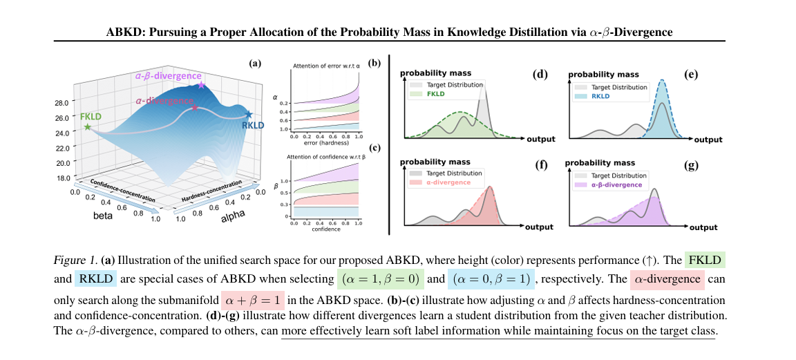
- Forward KL divergence spreads student probability too thinly across all classes, so the student fails to commit to the right answer.
- Reverse KL divergence does the opposite. It collapses the student onto one class and throws away the soft label information that made distillation valuable in the first place.
- The authors frame both failures through two effects they call hardness concentration and confidence concentration, and show that forward KL is weak in both while reverse KL is extreme in both.
- The alpha beta divergence generalizes both as special cases and lets you tune the two effects independently with two scalar hyperparameters.
- On five instruction following benchmarks, distilling GPT-2 XL into smaller GPT-2 variants, ABKD beats forward KL and reverse KL by 0.81 to 3.31 ROUGE-L points without touching the architecture or the training data.
- On CIFAR-100 and CLIP base to new transfer, ABKD acts as a drop in replacement for the loss in existing methods like DKD, LSD, and TTM and lifts each of them.
Why the standard recipe quietly breaks
Knowledge distillation has a clean story. A large teacher network outputs a probability distribution over classes, not a one hot label, and the student learns to match that distribution. Soft labels carry richer information than ground truth alone. The student should generalize better than it would from labels and inputs alone. That is the pitch Hinton, Vinyals, and Dean made in 2015 and it has held up across a decade of vision and language work.
The pitch hides a choice. To make student and teacher distributions match, you need a divergence. Almost every paper since 2015 picks the forward Kullback Leibler divergence, written as \( D_{KL}(p \| q_\theta) \), where p is the teacher and q the student. A smaller number of recent papers, especially in the large language model space, prefer reverse KL, written as \( D_{KL}(q_\theta \| p) \). The two look symmetric. They are not. They produce very different students.
Forward KL is mode covering. It punishes the student hard for assigning low probability to any class the teacher likes, including classes the teacher is only a little bit confident about. So the student spreads its probability mass to cover everything the teacher cares about. That sounds responsible. The problem is that with thousands of classes, like the 50,257 token vocabulary of GPT-2, spreading thin means never committing. Reverse KL does the opposite. It punishes the student for putting probability anywhere the teacher does not. The student learns to pick one mode and stay there. With one hot ground truth labels available anyway, the student often collapses onto the target class and throws away everything else the teacher had to say.
The pattern is well known empirically. Wen and colleagues noted it in 2023. Wu and colleagues confirmed it in 2024. Ko and colleagues built a whole streamlined distillation pipeline around it. The question Guanghui Wang and his coauthors ask is sharper. Why exactly do both extremes fail, and is there a principled middle ground that is not just a weighted average of two broken things?
Two concentration effects, one diagnosis
Here is where it gets interesting. The authors track what happens to the student probability of a class y across a single gradient step. They call this quantity the log mass ratio, the logarithm of \( q_{t+1}(y) / q_t(y) \), and they show it is proportional to the gradient of the loss with respect to the logit for class y. So watching the log mass ratio is the same as watching how the loss reshapes the student distribution one update at a time.
When you write the log mass ratio bound for forward KL, two factors fall out. There is a matching loss factor of the form \( |p(y) – q_t(y)| \), and there is a weighting factor that is just a constant 1. When you do the same for reverse KL, the matching loss factor becomes a logarithmic version, \( |\log p(y) – \log q_t(y)| \), and the weighting factor becomes \( q_t(y) \).
The authors give these two factors names that make the analysis click. The matching loss factor controls what they call hardness concentration. A sharper version of this factor pushes the student to fix the worst errors first, the classes where it is most wrong relative to the teacher. The weighting factor controls confidence concentration. A version that emphasizes high probability classes makes the student care mostly about getting right what it already thinks is right.
Think about what this actually means for the gradient. Under forward KL, every class with a mismatch contributes equally to the update. The student has no reason to prioritize the target class over irrelevant noise classes. Under reverse KL, the confidence weighting amplifies whatever the student already believes. Once the student has even a slight lean toward the target class, the gradient drives it further in that direction, and the soft label information from the teacher quietly disappears from the loss.
The authors prove a formal theorem that nails this down. Forward KL allocates mass changes across classes more or less uniformly. Reverse KL preferentially adds mass to underestimated classes that already have higher student probability, and preferentially removes mass from overestimated classes that have lower student probability. The small get smaller and the big get bigger. That is exactly the mode seeking behavior people complain about, derived from first principles instead of described from intuition.
The alpha beta divergence, an old idea put to a new use
The cure the authors reach for is a family of divergences introduced by Cichocki, Cruces, and Amari in 2011 for robust non negative matrix factorization. Define
The two scalars alpha and beta do the work. Set alpha to 1 and beta to 0 and the limit recovers forward KL. Set alpha to 0 and beta to 1 and the limit recovers reverse KL. The Hellinger distance sits at alpha equals beta equals 0.5. The squared Euclidean distance sits at alpha equals beta equals 1. So the family contains every distribution measure people have already tried in distillation as a special point in a two dimensional plane.
The reason this matters is what happens when you redo the log mass ratio analysis under the alpha beta divergence. The matching loss factor becomes \( |p(y)^\alpha – q_t(y)^\alpha| / \alpha \), and the weighting factor becomes \( q_t(y)^\beta \). Now alpha and beta separately control the two effects. A smaller alpha sharpens hardness concentration, making the gradient pay more attention to large errors. A larger beta sharpens confidence concentration, making the gradient pay more attention to classes the student already trusts. Crucially, the two knobs are independent.
Forward KL and reverse KL are not opposites. They are two corners of a rectangle, and the interior of the rectangle is where the good losses live. A way to read Wang and colleagues
This is a different proposition from the alpha divergence family proposed by Chernoff in 1952, which has appeared in a few distillation papers. Alpha divergence is one dimensional. It interpolates between forward and reverse KL along the line where alpha plus beta equals 1. So tightening hardness concentration forces you to loosen confidence concentration. The authors show that this constraint is exactly what stops alpha divergence from reaching the better region of the loss landscape. Two dimensions of freedom turn out to matter.
What does the proper allocation look like
To see the practical effect, the authors run sensitivity studies on both image classification and instruction following. The patterns are intuitive once you have the two effects in mind.
On CIFAR-100, where the output distribution lives over 100 classes, a relatively large alpha around 0.7 to 0.9 paired with a small beta around 0.2 to 0.5 works best. The output space is small enough that you do not need extreme hardness concentration. You just need a slight tilt toward error focus and a mild confidence weighting. On the Dolly instruction following benchmark, where the output distribution lives over the 50,257 token vocabulary, the recipe flips. A smaller alpha around 0.2 paired with a larger beta around 0.7 wins. With so many tokens, the student gets lost without aggressive hardness focus, and it needs strong confidence weighting to commit to plausible next tokens.
This is a rare case where the theory hands you a rule of thumb that practitioners can actually use. Inversely scale alpha with the difficulty of focusing on large errors, which roughly tracks the dimensionality of the output. Scale beta up when the output vocabulary is large and you need the student to commit, scale it down when the soft label structure across classes is the real signal.
The numbers, and what they actually show
The empirical scope is large. The authors evaluate across 17 language and vision datasets and 12 teacher and student configurations, with model sizes ranging from 0.46 million parameter convolutional networks to 1.5 billion parameter language models. The headline experiments distill GPT-2 XL at 1.5 billion parameters into smaller GPT-2 variants. Here is the picture on five instruction following benchmarks.
| Method | Dolly Eval | Self-Instruct | Vicuna Eval | Super-Natural | Unnatural |
|---|---|---|---|---|---|
| SFT only | 23.14 | 10.22 | 15.15 | 17.41 | 19.76 |
| Vanilla KD (forward KL) | 23.80 | 10.01 | 15.25 | 17.69 | 18.99 |
| SeqKD (Kim, Rush) | 24.28 | 11.24 | 14.94 | 20.66 | 23.59 |
| MiniLLM (reverse KL) | 24.62 | 12.49 | 17.30 | 23.76 | 24.30 |
| GKD (JS divergence) | 24.49 | 11.41 | 16.01 | 18.25 | 21.41 |
| DISTILLM (Ko et al.) | 25.32 | 11.65 | 16.76 | 23.52 | 25.79 |
| ABKD (this paper) | 25.65 | 13.47 | 16.06 | 26.47 | 29.32 |
The gains are not small. On Unnatural Instructions, ABKD jumps from 18.99 ROUGE-L under forward KL to 29.32, a 10.33 point improvement from changing nothing but the loss function. On Super-Natural the gain is 8.78 points. Three of the five datasets see the student match or exceed the teacher’s own ROUGE-L score, which is the kind of result that makes you check the table twice.
What makes the comparison fair is that ABKD uses the fixed training set, while several stronger baselines like MiniLLM, GKD, and DISTILLM also use student generated outputs, a data augmentation trick that costs 1.6 to 7 times more training time. The authors show in the appendix that combining ABKD with student generated outputs gives a further 0.4 to 1.6 point lift, so the loss function and the data strategy stack rather than substitute.
On image classification the story is similar in shape if smaller in size. On eight teacher and student pairs across CIFAR-100, ABKD lifts every backbone it is bolted onto, including DKD, LSD, and TTM, which are themselves strong recent distillation methods. The base to new transfer experiment with CLIP, where the student is trained on a set of base classes and evaluated on novel classes, gives ABKD a 0.38 to 0.54 point harmonic mean advantage over the best non distillation prompt tuning baselines. That margin is small in absolute terms but consistent across all 11 datasets, which is harder to fake.
Where the framework gets honest about its limits
No method earns trust without owning what it cannot do. The authors are reasonable about this and the careful reader should be too.
The two hyperparameters need tuning. The paper provides clear inductive bias rules and a sensitivity analysis, but there is no universal default. On a new task with an unusual output shape, you may need a small grid search. The authors argue this is cheap because each setting only changes the loss, not the training pipeline, but a grid is still a grid. For practitioners who want a single button, vanilla KD is still less work even if it leaves performance on the table.
The framework only changes the divergence. It does not address the deeper question of whether matching the teacher distribution is the right objective at all. DISTILLM, MiniLLM, and others argue that you should also rethink which sequences you train on, by sampling student generated outputs and getting teacher feedback on those. ABKD is orthogonal to this question and benefits from it, but does not answer it.
The instruction following gains are reported on relatively small teachers by current standards. GPT-2 XL is a 1.5 billion parameter model from 2019. The OpenLLaMA2-7B to 3B experiments in the appendix show the gains hold at a larger scale, with 0.65 to 3.26 ROUGE-L improvements over the strongest baselines, but the field has moved to 70 billion and 405 billion parameter teachers. The authors did not run those experiments, presumably for compute reasons, and so the asymptotic behavior at frontier scale is an open question.
The authors also acknowledge that for tasks with very low dimensional outputs, the alpha beta divergence may simplify back toward forward KL territory, with alpha near 1 and beta near 0. That is consistent with the theory and with the observation that on CIFAR-100, alpha settles at 0.7 to 0.9. The framework does not make every task harder. It just lets you reach the right corner of the rectangle when the task needs you to.
What this changes for practitioners
If you train students against soft teacher labels, the takeaway is concrete. Replace your KL loss with the alpha beta divergence loss and tune two scalars. For language modeling tasks with vocabularies in the tens of thousands, start with alpha around 0.2 and beta around 0.7. For image classification with class counts in the hundreds, start with alpha around 0.8 and beta around 0.3. Sweep a small grid from there. Do not change anything else first.
If you work on logit standardization, decoupled distillation, or transformed teacher matching, the alpha beta divergence is a drop in replacement for the KL inside your method. The authors show this with ABDKD, ABLSD, and ABTTM, all of which beat their forward KL parents on the same backbones. The loss and the higher level method compose cleanly, which is unusual.
If you build distillation pipelines that already use student generated outputs, the effects stack. ABKD plus the adaptive off policy strategy from DISTILLM gives the strongest numbers in the paper. Loss design and data design are different levers and you can pull both.
Reproducing ABKD in PyTorch
Here is a minimal reproduction. The class implements the alpha beta divergence with the continuous extensions that recover forward and reverse KL at the boundary, and a small training loop that runs against a dummy CIFAR like setup. The implementation tracks the paper’s formulation in Definition 4.1 and the gradient analysis in Lemma E.1.
Switch the alpha and beta in ABKDLoss to mimic forward KL with (1, 0), reverse KL with (0, 1), or Hellinger with (0.5, 0.5), and you can reproduce the special cases shown in Table 1 of the paper without changing the rest of the pipeline. The official implementation, with the full image and language experiments, is on GitHub at github.com/ghwang-s/abkd.
Conclusion
The cleanest result in this paper is conceptual. Knowledge distillation has been treated as a problem of choosing between forward KL and reverse KL, with various weighted averages, Jensen Shannon divergences, and adaptive schedules attempting to triangulate between them. Wang and his coauthors show that all of those approaches are walking along a single line in a larger space of losses, and that the line itself was the wrong primitive. The right primitive is a two dimensional region, with hardness concentration on one axis and confidence concentration on the other, and the two endpoints everyone has been arguing about are just two corners of that region.
The conceptual shift comes with mathematics that does real work. The alpha beta divergence is not a new family. It comes from a 2011 information geometry paper that did not have distillation in mind. Reapplying it here lights up an interpretation that the original work could not have anticipated. Forward and reverse KL are the boundary cases, alpha divergence carves out a one dimensional submanifold, and Hellinger and Euclidean distance sit at other corners. The framework is general enough to subsume what came before and tight enough to give specific hyperparameter recommendations.
The transferability is real. The same trick that works for instruction tuning GPT-2 also works for vision transformer prompt tuning, for ResNet to ResNet image classification distillation, and as a drop in replacement inside other methods. That breadth makes the method less of a clever benchmark hack and more of a primitive that may keep paying off. The gains do not require new architecture, new data, or new training tricks. They require swapping one loss function and tuning two scalars.
There are honest open questions. Whether the framework scales to 70 billion parameter teachers and what its compute trade off looks like at that scale are not yet answered. Whether the two hyperparameter formulation extends cleanly to feature based distillation or relational distillation, where the targets are not class probabilities, is an open direction. The connection the authors point out to direct preference optimization, where the same mode seeking behavior shows up under a different name, hints that the mass concentration framework might be a useful lens beyond distillation entirely.
The reason this paper matters is not that it claims a state of the art on every benchmark, though it does on many of them. It is that the diagnosis of why the standard recipe was failing is precise enough to be acted on, and the cure is light enough to be tested in an afternoon. If you train students against teachers, the alpha beta divergence is the kind of small change that pays its keep.
Frequently Asked Questions
What is the alpha beta divergence in plain terms?
It is a family of distance measures between two probability distributions, parameterized by two scalars alpha and beta. By picking different alpha and beta values, you recover forward KL divergence, reverse KL divergence, Hellinger distance, squared Euclidean distance, and many measures in between. In knowledge distillation it lets you tune how aggressively the student fixes large errors and how much it focuses on classes it already trusts, as two independent settings.
Why does forward KL fail in knowledge distillation?
Forward KL spreads student probability mass over every class the teacher has any belief in. With large output vocabularies this dilutes commitment to the right answer. The authors show that under forward KL the gradient treats matching errors on all classes equally, which gives the student no reason to prioritize the target class over irrelevant noise classes.
Why does reverse KL also fail?
Reverse KL collapses the student onto a small number of modes in the teacher distribution and often just onto the target class. That throws away the soft label structure that made distillation worthwhile in the first place. The math shows it preferentially grows mass on classes the student already favors, which is a self reinforcing trap.
How do you pick alpha and beta?
For tasks with high dimensional output distributions like language modeling over 50,000 tokens, the paper recommends a small alpha around 0.2 and a large beta around 0.7. For tasks with low dimensional outputs like image classification over 100 classes, a larger alpha around 0.7 to 0.9 and a smaller beta around 0.2 to 0.5 works better. A small grid search around these defaults is the recommended starting point.
Can I combine ABKD with methods like DKD, LSD, or DISTILLM?
Yes. The authors show that swapping the loss inside DKD gives ABDKD, inside LSD gives ABLSD, inside TTM gives ABTTM, and each variant beats its forward KL parent on the same architectures. The alpha beta divergence is orthogonal to the higher level distillation strategy and composes cleanly with student generated output augmentation as well.
How big are the gains over standard knowledge distillation?
On the five instruction following benchmarks where GPT-2 XL is distilled into GPT-2, ABKD beats vanilla forward KL by 0.81 to 10.33 ROUGE-L points, with the largest gain on Unnatural Instructions. On CIFAR-100 across eight teacher and student pairs, ABKD lifts every backbone it is applied to. On CLIP base to new transfer across 11 datasets it improves the harmonic mean accuracy over the best non distillation prompt tuning baseline by 0.38 to 0.54 points.
Read the full ABKD paper
The original paper has the full theoretical proofs, ablation tables, and the OpenLLaMA experiments at larger scale.
Read the arXiv paper Get the codeCitation. Wang, G., Yang, Z., Wang, Z., Wang, S., Xu, Q., and Huang, Q. (2025). ABKD, Pursuing a Proper Allocation of the Probability Mass in Knowledge Distillation via Alpha Beta Divergence. arXiv preprint arXiv:2505.04560v3. Available at https://arxiv.org/abs/2505.04560. Code available at https://github.com/ghwang-s/abkd.
This analysis is based on the published paper and an independent evaluation of its claims.
Pingback: 7 Revolutionary Breakthroughs in AI Disease Grading — The Good, the Bad, and the Future of UMKD - aitrendblend.com
I don’t think the title of your article matches the content lol. Just kidding, mainly because I had some doubts after reading the article. https://accounts.binance.com/sl/register-person?ref=I3OM7SCZ