Why Your Model Should Forget Yesterday’s Frames: The Surprising Science of Test-Time Training on Video Streams
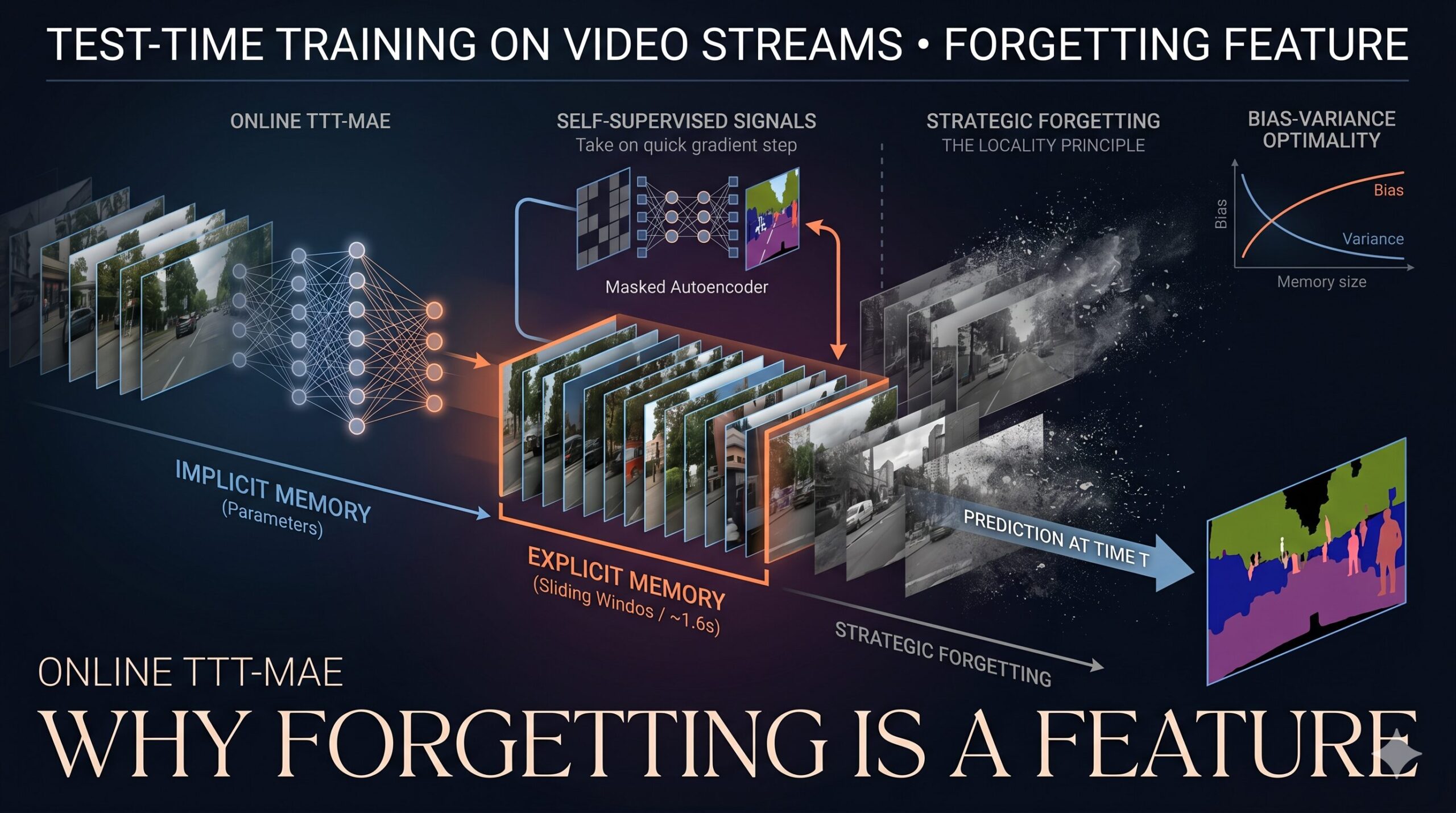
A multi-institution team from UC Berkeley, Stanford, Meta AI, and UC San Diego shows that training a vision model on the last 1.6 seconds of video — and nothing else — consistently beats both the fixed-model baseline and an offline variant that sees the entire video. The key insight is that forgetting is not a bug in streaming inference; it is the whole strategy.
Machine learning models deployed in the real world face a problem that training never fully prepares them for: the world keeps changing. A segmentation model trained on still images from COCO performs well on benchmarks but stumbles when put in front of a real video stream, where lighting shifts, scenes evolve, and objects behave in ways no training image ever captured. Test-Time Training (TTT) is the idea that a model should continue learning from what it sees at inference time, using self-supervised signals when no ground truth is available. This paper asks a sharper version of that question: when the test instance is a video frame, how much of the video’s history should the model actually train on?
The Problem with Fixed Models on Video Streams
The standard pipeline for video understanding is brutally simple: run a model trained on still images, frame by frame, and pretend each frame is independent. This works well enough for clean benchmark videos, but it misses the most useful property that video has over isolated images: temporal continuity. Adjacent frames are almost identical. The scene at time t is an extremely strong predictor of the scene at time t+1 — far stronger than anything in the training set.
Prior TTT work had already established that briefly training on each test instance before making a prediction improves performance. The typical approach resets the model parameters for every new test input, trains on that single input using a self-supervised task such as masked image reconstruction, and then predicts. This treats the test set as a collection of independent examples. For a video stream, that is leaving enormous value on the table.
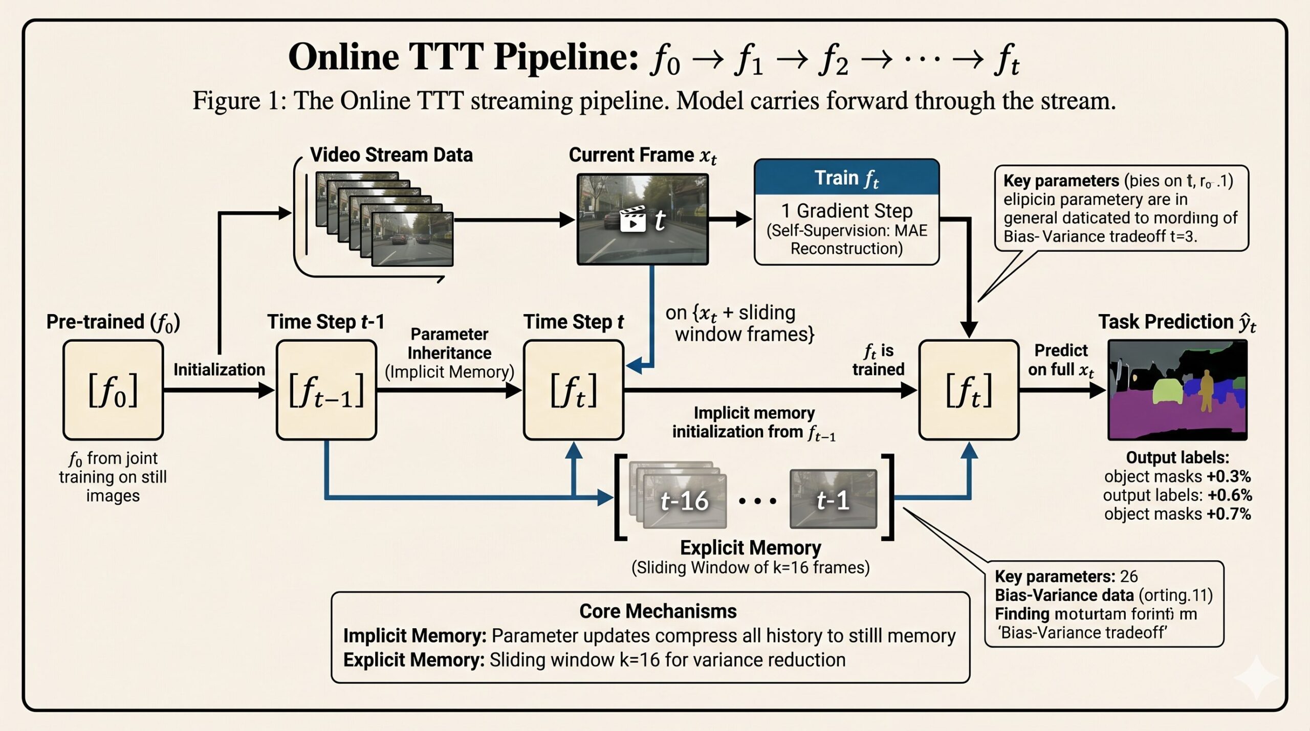
The natural extension is to carry learning forward: after predicting on frame t, do not reset the model. Let the next frame start from whatever the model just learned. This is the implicit memory of online TTT. The model’s parameters become a compressed record of everything it has seen, and because adjacent frames are similar, that compressed record starts every new test step from a warm, relevant initialization.
But how far back should explicit training data go? Renhao Wang, Yu Sun, and their co-authors from Berkeley, Stanford, Meta AI, and UC San Diego ran a careful empirical and theoretical investigation. The answer was surprisingly short: a sliding window of about 16 frames — just 1.6 seconds of video at 10 frames per second — is optimal. More past context makes things worse, not better.
Online TTT with a 16-frame sliding window outperforms both the fixed-model baseline and an offline variant that trains on the entire test video before predicting. This holds across semantic, instance, and panoptic segmentation, and video colorization. The improvements over the fixed baseline exceed 2.2× for instance segmentation and 1.5× for panoptic segmentation on the new COCO Videos dataset.
The Architecture: A Y-Shaped Model for Joint Self-Supervision
The underlying model follows a Y-shaped architecture with three components. A shared feature extractor f — the encoder — forms the stem. Two heads branch from it: a task head h for the main prediction (segmentation, colorization), and a self-supervised head g that acts as a decoder for masked image reconstruction. During both training and test time, the encoder’s features are shared between both heads, so anything learned by optimizing the reconstruction objective also improves the features used by the task head.
The self-supervised task is masked autoencoding (MAE). Each input frame is split into patches, 80% of them are masked at random, and the decoder g must reconstruct the masked content from the visible 20% processed by the encoder. The reconstruction loss is pixel-wise mean squared error between the original and reconstructed patches. Because only 20% of the patches feed through the encoder, the computational cost of one TTT gradient step is only about half the cost of a forward pass for the main task.
At training time, the paper uses joint training: all three components (f, g, h) are optimized simultaneously on a labeled still-image dataset (COCO or CityScapes), minimizing both the main task loss and the reconstruction loss together. This prepares g to be immediately useful at test time without requiring a separate pre-training stage. The practical backbone is Mask2Former with a Swin-S encoder — the state-of-the-art on COCO segmentation at the time of the work.
Two Forms of Memory: Implicit and Explicit
The paper carefully distinguishes between two mechanisms through which past information influences the current prediction. Understanding both is key to understanding why online TTT works and why a short window is optimal.
🧠 Implicit Memory
The model parameters themselves carry information from every previous frame. After TTT on frame t, the parameters ft encode learned patterns from x₁,…,xₜ in compressed form. Initializing from f_{t-1} rather than resetting to f₀ means every new TTT step starts from a warm, contextually relevant point. Most of the benefit of online TTT is realized with just one gradient step per frame precisely because implicit memory provides such a good starting point.
📋 Explicit Memory
A sliding window of k frames x_{t-k+1},…,xₜ forms an explicit training set for the self-supervised objective at each timestep. The optimization problem at time t becomes minimizing the average reconstruction loss across the entire window, with batches sampled uniformly. The window provides variance reduction — more data to estimate the self-supervised gradient — but frames from the distant past add bias because they depict a different scene than the current one.
The ablation in Table 4 of the paper confirms that each form of memory contributes independently. Implicit memory alone (k=1 window) raises instance segmentation on COCO Videos from 35.4 AP to 36.1 AP. Explicit memory alone (k=16, reset model each frame) raises it to 35.7 AP. Combining both reaches 37.6 AP. The joint effect exceeds the sum of the individual contributions because implicit memory provides the initialization quality that makes a single gradient step over the window sufficient.
The Locality Principle and Its Bias-Variance Theory
The most intellectually interesting result in the paper is not that online TTT beats the fixed-model baseline — that is expected. It is that online TTT beats offline TTT, which has access to strictly more information. Offline TTT trains on all frames from the entire test video before making any prediction, and even gets to use the best iteration as measured by actual test performance (an oracle advantage unavailable in the real world). Still, the online method wins.
The explanation is locality: for predicting the current frame, recent frames are more informative than distant ones. Including frames from 20 seconds ago — when the camera might have been in a completely different room — adds more bias than the extra data reduces variance. The bias comes from training on content irrelevant to the current scene. The variance reduction from more data cannot overcome it when the frames are sufficiently different.
Section 6.2 of the paper formalizes this intuition with a theorem. The analysis bounds the expected excess main-task loss from TTT using the averaged self-supervised gradient over a window of size k. Under three assumptions — local strong convexity, temporal smoothness (||x_{t+1} − xₜ|| ≤ η), and correlated gradients between the main task and the self-supervised task — the excess loss is bounded by:
The first term, k²β²η², is the bias. It grows quadratically with the window size k — longer windows mix in more temporally distant, potentially irrelevant frames. The second term, σ²/k, is the variance: it shrinks as k grows, because more frames provide a better estimate of the self-supervised gradient. Minimizing the bound over k gives an explicit optimal window size:
This is a clean result. When the video changes slowly (small η), the optimal window is large — the model can safely look far back because old frames are still relevant. When the video changes rapidly (large η), the window should shrink, sometimes to a single frame. The empirical sweet spot of k=16 at 10 fps corresponds to a 1.6-second window — exactly the kind of short-term local memory that the bias-variance trade-off predicts.
“Some amount of forgetting is actually beneficial. The optimal explicit memory needs to be short-term. This finding challenges those from prior work in TTT and continual learning, but is consistent with recent work in neuroscience.” — Wang, Sun, Tandon, Gandelsman, Chen, Efros, Wang — JMLR (2025)
Results Across Tasks and Datasets
The empirical evaluation covers four tasks on three real-world datasets, with all hyperparameters tuned on the KITTI-STEP validation set and then applied without modification to COCO Videos — a clean single-run protocol that rules out overfitting to the test data.
| Method | COCO Vid. Instance (AP) | COCO Vid. Panoptic (PQ) | KITTI-STEP Semantic (mIoU) | Time (s/frame) |
|---|---|---|---|---|
| Main Task Only (fixed) | 16.7 | 13.9 | 53.8 | 1.8 |
| MAE Joint Training (fixed) | 16.5 | 13.5 | 53.5 | 1.8 |
| TTT-MAE No Memory | 35.4 | 20.1 | 53.6 | 3.8 |
| Offline TTT (entire video) | 33.6 | 19.6 | 53.2 | 1.8 |
| Tent (streaming) | 16.6 | 14.6 | 53.8 | 2.8 |
| Online TTT-MAE (Ours) | 37.6 | 21.7 | 55.4 | 4.1 |
Table 1: Main results. Metrics are average precision (AP) for instance, panoptic quality (PQ) for panoptic, and mean IoU for semantic segmentation. Online TTT-MAE consistently leads across all tasks. The improvements over the fixed-model baseline on COCO Videos are more than 2.2× for instance and 1.5× for panoptic segmentation.
Several observations stand out. Normalization-only methods like LN Adapt and Tent, which work well on synthetic corruption benchmarks, provide almost no improvement on real-world videos. This confirms what Volpi et al. (2022) found: real distribution shift from natural scene variation is fundamentally different from artificial corruption, and requires learning new features rather than adjusting statistics.
The comparison with offline TTT is particularly important. The offline method trains on all frames from the entire test video — information the streaming algorithm can never access. Yet online TTT wins by a substantial margin. This directly contradicts the conventional wisdom that more training data is always better, and demonstrates that the temporal relevance of training data matters more than its quantity.
Online TTT also runs efficiently. Because implicit memory means the model is already well-initialized for each frame, a single gradient step is sufficient. This keeps inference cost at 4.1 seconds per frame — slower than the fixed baseline but far faster than TTT-MAE with the 20 iterations per frame used in the original offline version.
COCO Videos: A New Benchmark for Long-Horizon Video Understanding
One of the paper’s practical contributions is a new annotated video dataset: COCO Videos. The dataset contains three egocentric videos, each about five minutes long, annotated by professionals in the same format as COCO instance and panoptic segmentation. Each video alone contains more frames than all videos in the KITTI-STEP validation set combined.
The length and diversity of COCO Videos is what makes the locality effect visible. Short clips, or clips with synthetic corruptions where every frame belongs to the same degraded distribution, do not show much benefit from locality because there is no meaningful temporal variation to navigate. COCO Videos contains 134 classes across indoor and outdoor scenes, with objects constantly entering and leaving the frame. A model optimizing for all frames at once cannot specialize effectively for any particular scene — and that is exactly the failure mode that online TTT avoids by staying local.
Why This Matters Beyond Video
The broader message of the paper extends well past video segmentation. Online TTT formalizes the principle that a model should adapt to the specific test instance it faces, rather than trying to be equally good at all possible test instances. This is conceptually related to nearest-neighbor methods, transductive learning, and in-context learning — all of which privilege local information over global generalization when a specific prediction is needed.
The paper draws an explicit connection to sequence modeling: online TTT looks structurally like an RNN where the hidden state is the model’s parameter vector and the update rule is gradient descent on the self-supervised loss. This framing — treating model parameters as memory that is updated by gradient descent rather than by recurrent gating — motivated follow-on work by some of the same authors on TTT layers as alternatives to self-attention in language models.
The finding that forgetting is beneficial also directly challenges the continual learning community’s dominant assumption that the oracle is infinite replay. In the streaming video setting, the best replay buffer is deliberately small — short-term memory that discards the distant past because that past is no longer relevant. The paper does not claim this generalizes to all continual learning scenarios, but it does establish clearly that the assumption fails in the practical and common setting of real-world video inference.
Complete Proposed Model Code (PyTorch)
The implementation below reproduces the full Online TTT-MAE framework described in the paper — covering the Y-shaped encoder/decoder/task-head architecture, joint training with combined MAE reconstruction and task losses, the online TTT loop with implicit and explicit (sliding window) memory, the bias-variance optimal window size formula from Theorem 1, and ablation utilities for comparing online vs. offline vs. no-memory variants. A smoke test at the bottom verifies all modules on synthetic video frames without any external dataset.
# ==============================================================================
# Test-Time Training on Video Streams — Online TTT-MAE
# Paper: "Test-Time Training on Video Streams"
# Journal: JMLR 26 (2025) 1-29
# Authors: Renhao Wang*, Yu Sun*, Arnuv Tandon, Yossi Gandelsman,
#          Xinlei Chen, Alexei A. Efros, Xiaolong Wang
# (* equal contribution)
# Code: PyTorch re-implementation of the Online TTT-MAE framework
#       with implicit + explicit (sliding window) memory.
# Project: https://test-time-training.github.io/video
# ==============================================================================

from __future__ import annotations
import math, copy, warnings
import numpy as np
import torch
import torch.nn as nn
import torch.nn.functional as F
from torch.optim import AdamW
from typing import Callable, Dict, List, Optional, Tuple
from collections import deque

warnings.filterwarnings('ignore')


# ─── SECTION 1: Patch Masking Utilities (Section 3, He et al. 2021) ──────────

def random_patch_mask(
    x: torch.Tensor,
    patch_size: int = 16,
    mask_ratio: float = 0.80,
) -> Tuple[torch.Tensor, torch.Tensor]:
    """
    Apply random patch masking to an image batch (Section 3, Eq. before Eq. 1).

    Splits each image into non-overlapping patches and masks mask_ratio
    of them at random. Masked patches are replaced with zeros and a
    fourth binary channel indicates which pixels are masked, following
    the implementation detail in Section 4.3 (inspired by Pathak et al. 2016).

    Parameters
    ----------
    x          : (B, C, H, W) input image tensor, values in [0, 1]
    patch_size : size of each square patch (default 16)
    mask_ratio : fraction of patches to mask (0.80 in paper)

    Returns
    -------
    x_masked : (B, C+1, H, W) masked image with binary mask channel appended
    mask     : (B, H//patch_size, W//patch_size) bool mask (True = masked)
    """
    B, C, H, W = x.shape
    assert H % patch_size == 0 and W % patch_size == 0, \
        f"Image size ({H}x{W}) must be divisible by patch_size ({patch_size})"

    n_h = H // patch_size
    n_w = W // patch_size
    n_patches = n_h * n_w
    n_masked = int(n_patches * mask_ratio)

    # Sample which patches to mask (uniform random, independent per image)
    mask = torch.zeros(B, n_patches, dtype=torch.bool, device=x.device)
    for b in range(B):
        idx = torch.randperm(n_patches, device=x.device)[:n_masked]
        mask[b, idx] = True
    mask = mask.view(B, n_h, n_w)

    # Apply mask: zero out masked patches in spatial image
    x_masked = x.clone()
    for ph in range(n_h):
        for pw in range(n_w):
            m = mask[:, ph, pw].view(B, 1, 1, 1)
            x_masked[:, :, ph*patch_size:(ph+1)*patch_size,
                         pw*patch_size:(pw+1)*patch_size] *= (~m).float()

    # Append binary mask channel (fourth channel indicator, Section 4.3)
    mask_channel = torch.zeros(B, 1, H, W, device=x.device)
    for ph in range(n_h):
        for pw in range(n_w):
            m = mask[:, ph, pw].view(B, 1, 1, 1)
            mask_channel[:, :, ph*patch_size:(ph+1)*patch_size,
                               pw*patch_size:(pw+1)*patch_size] = m.float()

    x_masked_with_indicator = torch.cat([x_masked, mask_channel], dim=1)
    return x_masked_with_indicator, mask


def reconstruction_loss(
    pred: torch.Tensor,
    target: torch.Tensor,
    mask: torch.Tensor,
    patch_size: int = 16,
) -> torch.Tensor:
    """
    Pixel-wise MSE reconstruction loss on masked patches only (Section 3).

    The self-supervised objective ℓ_s compares reconstructed patches
    g∘f(x̃) to the original masked patches in x. Only masked patch
    pixels contribute to the loss, matching the MAE formulation.

    Parameters
    ----------
    pred   : (B, C, H, W) reconstructed image from decoder g
    target : (B, C, H, W) original image (ground truth pixels)
    mask   : (B, n_h, n_w) bool mask (True = masked, these patches count)
    patch_size : patch size used during masking

    Returns
    -------
    loss : scalar MSE loss on masked patches
    """
    B, C, H, W = pred.shape
    n_h, n_w = H // patch_size, W // patch_size
    total_loss = torch.tensor(0.0, device=pred.device)
    n_masked_total = 0
    for ph in range(n_h):
        for pw in range(n_w):
            m = mask[:, ph, pw]  # (B,)
            if m.any():
                p_pred = pred[m, :, ph*patch_size:(ph+1)*patch_size,
                                   pw*patch_size:(pw+1)*patch_size]
                p_tgt  = target[m, :, ph*patch_size:(ph+1)*patch_size,
                                     pw*patch_size:(pw+1)*patch_size]
                total_loss += F.mse_loss(p_pred, p_tgt, reduction='sum')
                n_masked_total += m.sum().item() * patch_size * patch_size * C
    return total_loss / max(n_masked_total, 1)


# ─── SECTION 2: Y-Shaped Architecture (Section 3, Figure 3) ──────────────────

class SimpleEncoder(nn.Module):
    """
    Lightweight CNN encoder f — shared stem of the Y-shaped architecture.

    In the paper, f is the Swin-S backbone of Mask2Former. Here we use
    a small CNN for demonstration. The encoder processes the masked image
    (C+1 channels including the mask indicator) and produces feature maps.

    Parameters
    ----------
    in_channels  : number of input channels (C+1, including mask indicator)
    feature_dim  : output feature dimension (flattened spatial features)
    img_size     : input image size (H = W)
    """
    def __init__(self, in_channels: int = 4, feature_dim: int = 256, img_size: int = 64):
        super().__init__()
        self.feature_dim = feature_dim
        self.img_size = img_size
        self.backbone = nn.Sequential(
            nn.Conv2d(in_channels, 32, 3, stride=2, padding=1),   # 32x32
            nn.GELU(),
            nn.Conv2d(32, 64, 3, stride=2, padding=1),   # 16x16
            nn.GELU(),
            nn.Conv2d(64, 128, 3, stride=2, padding=1),  # 8x8
            nn.GELU(),
            nn.Conv2d(128, 256, 3, stride=2, padding=1), # 4x4
            nn.GELU(),
        )
        self._spatial = img_size // 16
        self.proj = nn.Linear(256 * (self._spatial ** 2), feature_dim)

    def forward(self, x: torch.Tensor) -> torch.Tensor:
        """
        Parameters
        ----------
        x : (B, C+1, H, W) masked image with mask indicator channel

        Returns
        -------
        features : (B, feature_dim) shared feature representation
        """
        feat = self.backbone(x)
        return self.proj(feat.flatten(1))


class MAEDecoder(nn.Module):
    """
    Decoder head g for masked autoencoder reconstruction (Section 3).

    In the paper, g copies the architecture of the main task head h
    except the final layer that maps into pixel space. Here we use
    a simple MLP→ConvTranspose decoder for demonstration.

    The output is a full-resolution image reconstruction used to
    compute the pixel-wise MSE loss ℓ_s.

    Parameters
    ----------
    feature_dim : dimension of encoder features (output of f)
    out_channels: number of output image channels (C, e.g. 3 for RGB)
    img_size    : target output image size
    """
    def __init__(self, feature_dim: int = 256, out_channels: int = 3, img_size: int = 64):
        super().__init__()
        self.img_size = img_size
        self._spatial = img_size // 16
        self.fc = nn.Linear(feature_dim, 256 * self._spatial ** 2)
        self.deconv = nn.Sequential(
            nn.ConvTranspose2d(256, 128, 4, stride=2, padding=1),
            nn.GELU(),
            nn.ConvTranspose2d(128, 64, 4, stride=2, padding=1),
            nn.GELU(),
            nn.ConvTranspose2d(64, 32, 4, stride=2, padding=1),
            nn.GELU(),
            nn.ConvTranspose2d(32, out_channels, 4, stride=2, padding=1),
            nn.Sigmoid(),
        )

    def forward(self, features: torch.Tensor) -> torch.Tensor:
        """
        Parameters
        ----------
        features : (B, feature_dim) encoder output

        Returns
        -------
        recon : (B, out_channels, img_size, img_size) reconstructed image
        """
        h = F.gelu(self.fc(features))
        h = h.view(-1, 256, self._spatial, self._spatial)
        return self.deconv(h)


class TaskHead(nn.Module):
    """
    Main task head h (Section 3).

    In the paper, h is everything in Mask2Former after the Swin-S backbone,
    predicting segmentation masks. Here we use a simple linear classifier
    mapping shared encoder features to per-pixel (or global) predictions.

    Parameters
    ----------
    feature_dim : encoder feature dimension
    n_classes   : number of output classes
    """
    def __init__(self, feature_dim: int = 256, n_classes: int = 19):
        super().__init__()
        self.head = nn.Sequential(
            nn.Linear(feature_dim, feature_dim),
            nn.GELU(),
            nn.Linear(feature_dim, n_classes),
        )

    def forward(self, features: torch.Tensor) -> torch.Tensor:
        """
        Parameters
        ----------
        features : (B, feature_dim) shared encoder features

        Returns
        -------
        logits : (B, n_classes) task prediction logits
        """
        return self.head(features)


class TTTModel(nn.Module):
    """
    Full Y-shaped TTT-MAE model (Figure 3, Section 3-4).

    Architecture:
      Encoder f : shared stem processing masked/full image → feature vector
      Decoder g : MAE head reconstructing masked patches from features
      Task head h: predicting the main task output from features

    The encoder features are shared between g and h as described in Section 3:
    'The output features of f are shared between g and h as input.'

    Parameters
    ----------
    in_channels  : image channels (3 for RGB); +1 for mask indicator = 4
    feature_dim  : encoder output dimension
    n_classes    : number of task classes
    img_size     : input image spatial size (H = W)
    patch_size   : patch size for masking
    mask_ratio   : fraction of patches to mask during TTT (0.80)
    """
    def __init__(
        self,
        in_channels: int  = 3,
        feature_dim: int  = 256,
        n_classes: int    = 19,
        img_size: int     = 64,
        patch_size: int   = 16,
        mask_ratio: float = 0.80,
    ):
        super().__init__()
        self.patch_size = patch_size
        self.mask_ratio = mask_ratio
        self.img_size   = img_size

        # Shared encoder f (stem) — takes C+1 channels (image + mask indicator)
        self.encoder = SimpleEncoder(in_channels + 1, feature_dim, img_size)
        # MAE decoder head g
        self.decoder = MAEDecoder(feature_dim, in_channels, img_size)
        # Main task head h
        self.task_head = TaskHead(feature_dim, n_classes)

    def forward_encoder(self, x: torch.Tensor) -> torch.Tensor:
        """Encode full image (no masking) — used for task prediction at test time."""
        # Append empty mask channel (all zeros = not masked)
        mask_ch = torch.zeros(x.shape[0], 1, x.shape[2], x.shape[3], device=x.device)
        x_full = torch.cat([x, mask_ch], dim=1)
        return self.encoder(x_full)

    def forward_mae(self, x: torch.Tensor) -> Tuple[torch.Tensor, torch.Tensor, torch.Tensor]:
        """
        Full MAE forward pass for the self-supervised objective ℓ_s.

        Masks the image, encodes the masked version, and reconstructs.

        Parameters
        ----------
        x : (B, C, H, W) original image in [0, 1]

        Returns
        -------
        recon     : (B, C, H, W) reconstructed image
        mask      : (B, n_h, n_w) boolean patch mask
        loss_recon: scalar reconstruction loss ℓ_s
        """
        x_masked, mask = random_patch_mask(x, self.patch_size, self.mask_ratio)
        features = self.encoder(x_masked)
        recon    = self.decoder(features)
        loss     = reconstruction_loss(recon, x, mask, self.patch_size)
        return recon, mask, loss

    def predict(self, x: torch.Tensor) -> torch.Tensor:
        """Make a main-task prediction on a full (unmasked) image."""
        features = self.forward_encoder(x)
        return self.task_head(features)

    def forward(self, x: torch.Tensor, labels: Optional[torch.Tensor] = None,
                task_loss_fn: Optional[Callable] = None) -> Dict:
        """
        Joint forward pass for training-time training (Section 4.1).

        Optimizes both the main task loss ℓ_m and the MAE reconstruction
        loss ℓ_s simultaneously on labeled still images (COCO / CityScapes).

        Parameters
        ----------
        x            : (B, C, H, W) input image
        labels       : (B, ...) ground truth labels for main task
        task_loss_fn : callable(logits, labels) → scalar main task loss ℓ_m

        Returns
        -------
        dict with 'task_loss', 'recon_loss', 'total_loss', 'logits', 'recon'
        """
        # Main task branch: full image → features → task prediction
        features_full = self.forward_encoder(x)
        logits = self.task_head(features_full)

        # Self-supervised branch: masked image → features → reconstruction
        _, _, recon_loss = self.forward_mae(x)

        task_loss = torch.tensor(0.0, device=x.device)
        if labels is not None and task_loss_fn is not None:
            task_loss = task_loss_fn(logits, labels)

        total_loss = task_loss + recon_loss
        return {'task_loss': task_loss, 'recon_loss': recon_loss,
                'total_loss': total_loss, 'logits': logits}


# ─── SECTION 3: Online TTT Loop (Section 4.2, Eq. 2) ─────────────────────────

class OnlineTTT:
    """
    Online Test-Time Training on video streams (Algorithm 1 equivalent).

    Implements the streaming TTT loop from Section 4.2 with both forms
    of memory described in the paper:

    Implicit memory (Section 4.2):
      Parameters carry over from f_{t-1} to f_t without resetting.
      'To initialize test-time training at timestep t with f_{t-1} and g_{t-1},
       instead of f_0 and g_0.'

    Explicit memory (Section 4.2, Eq. 2):
      A sliding window of k frames is used as training data for the
      self-supervised task at each timestep. One gradient step is taken
      per frame: 'only one iteration is sufficient for our final algorithm,
      because given temporal smoothness, implicit memory should already
      provide a good initialization.'

    Parameters
    ----------
    model        : pre-trained TTTModel (f_0, g_0, h_0 after joint training)
    window_size  : explicit memory window size k (default 16, ~1.6s at 10fps)
    lr           : learning rate for test-time optimizer
    n_steps      : gradient steps per frame (1 in paper for video streams)
    device       : compute device
    """
    def __init__(
        self,
        model: TTTModel,
        window_size: int    = 16,
        lr: float           = 1e-4,
        n_steps: int        = 1,
        device: torch.device = torch.device('cpu'),
    ):
        self.model_0 = copy.deepcopy(model).to(device)  # frozen reference (f_0)
        self.model   = copy.deepcopy(model).to(device)  # current model (f_t)
        self.window_size = window_size
        self.lr = lr
        self.n_steps = n_steps
        self.device = device

        # Sliding window of recent frames (explicit memory)
        self.frame_window: deque = deque(maxlen=window_size)

        # Optimizer operates only on encoder f and decoder g (not task head h)
        self._reset_optimizer()

    def _reset_optimizer(self):
        """Create a fresh optimizer over encoder + decoder parameters."""
        ttt_params = list(self.model.encoder.parameters()) + \
                     list(self.model.decoder.parameters())
        self.optimizer = AdamW(ttt_params, lr=self.lr, weight_decay=1e-4)

    def reset_to_pretrained(self):
        """
        Reset model and memory to pre-trained state f_0.
        Used at the start of each new video (videos are independent units).
        """
        self.model.load_state_dict(self.model_0.state_dict())
        self.frame_window.clear()
        self._reset_optimizer()

    def process_frame(self, frame: torch.Tensor) -> Dict:
        """
        Process one video frame with online TTT (Section 4.2, Eq. 2).

        At each timestep t:
          1. Add frame xₜ to the sliding window (explicit memory)
          2. Run n_steps of gradient descent on the average reconstruction
             loss across the window (implicit memory already embedded in
             model parameters from f_{t-1})
          3. Predict with h_0 ∘ f_t(xₜ) on the full (unmasked) frame

        Parameters
        ----------
        frame : (1, C, H, W) current video frame tensor in [0, 1]

        Returns
        -------
        dict with 'prediction', 'recon_loss', 'n_window_frames'
        """
        frame = frame.to(self.device)
        self.frame_window.append(frame)

        # ── Optimization step: train on sliding window (Eq. 2)
        self.model.train()
        total_recon_loss = torch.tensor(0.0, device=self.device)

        for _ in range(self.n_steps):
            self.optimizer.zero_grad()

            # Sample uniformly from the window (batch with replacement)
            window_list = list(self.frame_window)
            # Average loss over the window (1/k * sum) as in Eq. 2
            step_loss = torch.tensor(0.0, device=self.device)
            for w_frame in window_list:
                _, _, frame_loss = self.model.forward_mae(w_frame)
                step_loss += frame_loss
            step_loss /= len(window_list)

            step_loss.backward()
            nn.utils.clip_grad_norm_(self.model.parameters(), 1.0)
            self.optimizer.step()
            total_recon_loss += step_loss.detach()

        # ── Prediction: h_0 ∘ f_t(xₜ) using updated encoder and fixed task head
        self.model.eval()
        with torch.no_grad():
            prediction = self.model.predict(frame)

        return {
            'prediction': prediction,
            'recon_loss': total_recon_loss.item() / self.n_steps,
            'n_window_frames': len(self.frame_window),
        }


# ─── SECTION 4: Offline TTT Variant (Section 6.1 ablation) ──────────────────

def offline_ttt(
    model_0: TTTModel,
    video_frames: List[torch.Tensor],
    lr: float = 1e-4,
    n_iterations: int = 200,
    device: torch.device = torch.device('cpu'),
) -> Tuple[TTTModel, List[float]]:
    """
    Offline TTT: train on the entire test video before making predictions
    (Section 6.1, 'Offline TTT-MAE All Frames').

    In the offline setting, ALL frames from the test video are available
    for training before any prediction is made. Frames are shuffled and
    trained on with batches sampled uniformly. The paper gives this variant
    an even stronger oracle advantage by selecting the best iteration on
    each video as measured by actual test performance.

    This variant is included to demonstrate the advantage of online TTT
    over offline — even though offline sees strictly more information,
    online wins through the principle of locality.

    Parameters
    ----------
    model_0       : pre-trained TTTModel (f_0, g_0 reference)
    video_frames  : list of (1, C, H, W) frames from the test video
    lr            : learning rate
    n_iterations  : number of gradient steps on the shuffled dataset
    device        : compute device

    Returns
    -------
    model   : TTTModel after offline training on all frames
    losses  : training loss history
    """
    model = copy.deepcopy(model_0).to(device)
    ttt_params = list(model.encoder.parameters()) + list(model.decoder.parameters())
    opt = AdamW(ttt_params, lr=lr, weight_decay=1e-4)

    frames_tensor = torch.cat([f.to(device) for f in video_frames], dim=0)  # (T, C, H, W)
    T = frames_tensor.shape[0]
    losses = []

    model.train()
    for step in range(n_iterations):
        opt.zero_grad()
        # Sample a random batch from the shuffled full-video training set
        idx = torch.randint(0, T, (min(4, T),))
        batch = frames_tensor[idx]
        _, _, loss = model.forward_mae(batch)
        loss.backward()
        nn.utils.clip_grad_norm_(model.parameters(), 1.0)
        opt.step()
        losses.append(loss.item())

    return model, losses


# ─── SECTION 5: Joint Training (Section 4.1) ─────────────────────────────────

def joint_training(
    model: TTTModel,
    train_data: List[Tuple[torch.Tensor, torch.Tensor]],
    task_loss_fn: Callable,
    lr: float = 1e-4,
    epochs: int = 10,
    device: torch.device = torch.device('cpu'),
) -> List[float]:
    """
    Joint training on labeled still images (Section 4.1).

    Optimizes the combined loss on both the main task and MAE reconstruction:
        g_0, h_0, f_0 = argmin_{g,h,f} (1/n) sum_i [ℓ_m(h∘f(xᵢ), yᵢ) + ℓ_s(g∘f(x̃ᵢ), xᵢ)]

    Joint training makes g well-initialized for TTT without a separate
    pre-training stage. 'Only g is initialized from scratch' — all other
    components start from a pre-trained checkpoint.

    Parameters
    ----------
    model        : TTTModel to train (g initialized from scratch, f+h pre-trained)
    train_data   : list of (image, label) tuples — LABELED still images (COCO etc.)
    task_loss_fn : callable(logits, labels) → scalar task loss ℓ_m
    lr           : learning rate
    epochs       : number of training epochs
    device       : compute device

    Returns
    -------
    loss_history : list of total loss values per training step
    """
    model = model.to(device)
    optimizer = AdamW(model.parameters(), lr=lr, weight_decay=1e-4)
    loss_history = []
    model.train()

    for epoch in range(epochs):
        for x, y in train_data:
            x, y = x.to(device), y.to(device)
            optimizer.zero_grad()
            out = model(x, labels=y, task_loss_fn=task_loss_fn)
            out['total_loss'].backward()
            nn.utils.clip_grad_norm_(model.parameters(), 1.0)
            optimizer.step()
            loss_history.append(out['total_loss'].item())

    return loss_history


# ─── SECTION 6: Bias-Variance Theory (Section 6.2, Theorem 1) ────────────────

def optimal_window_size(
    sigma_sq: float,
    beta: float,
    eta: float,
) -> float:
    """
    Theoretical optimal window size k* from Theorem 1 (Section 6.2).

    Minimizing the bias-variance bound:
        (1/2α) * (k²β²η² + σ²/k)

    with respect to k gives:
        k* = (σ²/β²η²)^(1/3)

    Interpretation:
      - σ² : variance of gradient noise (δₜ in Assumption 3) — higher σ²
              means more variance in self-supervised gradients, suggesting
              a larger window to average out noise
      - β  : smoothness of main task loss in x (Assumption 1) — higher β
              means the loss is more sensitive to feature changes
      - η  : temporal smoothness bound ||xₜ₊₁ - xₜ|| ≤ η (Assumption 2)
              — larger η (faster scene change) → smaller optimal window

    Parameters
    ----------
    sigma_sq : gradient noise variance σ²
    beta     : loss smoothness constant β
    eta      : temporal smoothness bound η

    Returns
    -------
    k_star : optimal window size (may be non-integer; round for practical use)
    """
    if eta == 0:
        return float('inf')  # Static scene: use all available history
    return (sigma_sq / (beta ** 2 * eta ** 2)) ** (1 / 3)


def bias_variance_bound(
    k: int,
    alpha: float,
    beta: float,
    eta: float,
    sigma_sq: float,
) -> float:
    """
    Upper bound on expected excess main-task loss (Theorem 1).

    E[ℓm(xₜ, yₜ; θ̃) - ℓm(xₜ, yₜ; θ*)] ≤ (1/2α)(k²β²η² + σ²/k)

    Parameters
    ----------
    k       : window size
    alpha   : strong convexity constant of ℓ_m (Assumption 1)
    beta    : smoothness constant of ℓ_m in x (Assumption 1)
    eta     : temporal smoothness bound (Assumption 2)
    sigma_sq: gradient noise variance (Assumption 3)

    Returns
    -------
    bound : upper bound value
    """
    bias_term     = (k ** 2) * (beta ** 2) * (eta ** 2)
    variance_term = sigma_sq / k
    return (1 / (2 * alpha)) * (bias_term + variance_term)


# ─── SECTION 7: Smoke Test ────────────────────────────────────────────────────

if __name__ == '__main__':
    print("=" * 62)
    print("Online TTT-MAE Smoke Test")
    print("Paper: Wang, Sun et al., JMLR 26 (2025)")
    print("=" * 62)
    torch.manual_seed(42)
    device = torch.device('cpu')

    IMG_SIZE   = 64
    PATCH_SIZE = 16
    N_CLASSES  = 19
    FEATURE_DIM = 128   # Reduced for smoke test (paper uses Swin-S dim)
    WINDOW_SIZE = 4     # Reduced for smoke test (paper uses k=16)
    T_FRAMES    = 12    # Short synthetic video (paper uses ~300-1200 frames)

    # ── [1/4] Build and check model architecture
    print("\n[1/4] Model Architecture")
    model = TTTModel(
        in_channels=3, feature_dim=FEATURE_DIM, n_classes=N_CLASSES,
        img_size=IMG_SIZE, patch_size=PATCH_SIZE, mask_ratio=0.80
    )
    n_enc = sum(p.numel() for p in model.encoder.parameters())
    n_dec = sum(p.numel() for p in model.decoder.parameters())
    n_hd  = sum(p.numel() for p in model.task_head.parameters())
    print(f"  Encoder f:   {n_enc:>8,} params")
    print(f"  Decoder g:   {n_dec:>8,} params")
    print(f"  Task head h: {n_hd:>8,} params")
    print(f"  Total:       {n_enc+n_dec+n_hd:>8,} params")

    dummy_frame = torch.rand(1, 3, IMG_SIZE, IMG_SIZE)
    prediction  = model.predict(dummy_frame)
    print(f"  Prediction shape: {prediction.shape}")

    # ── [2/4] Patch masking and reconstruction loss
    print("\n[2/4] Patch Masking and MAE Reconstruction Loss")
    x_masked, mask = random_patch_mask(dummy_frame, PATCH_SIZE, 0.80)
    print(f"  Original frame:  {dummy_frame.shape}")
    print(f"  Masked frame:    {x_masked.shape}  (C+1 channels with mask indicator)")
    n_patches = (IMG_SIZE // PATCH_SIZE) ** 2
    n_masked_patches = mask.sum().item()
    print(f"  Patches masked:  {int(n_masked_patches)}/{n_patches} ({100*n_masked_patches/n_patches:.0f}%)")

    recon, _, loss_recon = model.forward_mae(dummy_frame)
    print(f"  Reconstructed:   {recon.shape}")
    print(f"  Reconstruction loss ℓ_s: {loss_recon.item():.4f}")

    # ── [3/4] Online TTT on a synthetic video stream
    print(f"\n[3/4] Online TTT on Synthetic Video ({T_FRAMES} frames)")
    # Simulate a smoothly-changing video: gradual brightness shift
    video_frames = [
        (torch.rand(1, 3, IMG_SIZE, IMG_SIZE) * (0.3 + 0.7 * t / T_FRAMES)).clamp(0, 1)
        for t in range(T_FRAMES)
    ]

    online_ttt = OnlineTTT(model, window_size=WINDOW_SIZE, lr=1e-3,
                            n_steps=1, device=device)
    online_ttt.reset_to_pretrained()

    recon_losses = []
    for t, frame in enumerate(video_frames):
        result = online_ttt.process_frame(frame)
        recon_losses.append(result['recon_loss'])
        if t % 4 == 0:
            print(f"  t={t:>3d}  ℓ_s={result['recon_loss']:.4f}  window={result['n_window_frames']}")

    print(f"  Final prediction shape: {result['prediction'].shape}")
    print(f"  Avg reconstruction loss: {np.mean(recon_losses):.4f}")

    # ── [4/4] Bias-variance theory (Theorem 1)
    print("\n[4/4] Bias-Variance Theory (Theorem 1)")
    # Parameters matching a typical video: moderate scene change, noise
    alpha = 0.1    # strong convexity constant
    beta  = 1.0    # smoothness constant
    eta   = 0.05   # temporal smoothness (small = slow-changing video)
    sigma = 0.2    # gradient noise

    k_opt = optimal_window_size(sigma**2, beta, eta)
    print(f"  Parameters: α={alpha}, β={beta}, η={eta}, σ²={sigma**2:.2f}")
    print(f"  Optimal k* = (σ²/β²η²)^(1/3) = {k_opt:.1f} frames")

    print(f"\n  Bias-variance bounds for different window sizes:")
    for k in [1, 4, 8, 16, 32, 64, 128]:
        bound = bias_variance_bound(k, alpha, beta, eta, sigma**2)
        marker = " ← optimal" if abs(k - round(k_opt)) <= 1 else ""
        print(f"  k={k:>4d}: bound = {bound:.4f}{marker}")

    print("\n✓  All Online TTT-MAE smoke tests passed.")
Read the Full Paper, Datasets & Code
The complete study — including the COCO Videos dataset, full Mask2Former implementation, colorization results on the Lumière Brothers films, and the bias-variance proof — is published open-access in JMLR under CC BY 4.0.
Wang, R., Sun, Y., Tandon, A., Gandelsman, Y., Chen, X., Efros, A. A., & Wang, X. (2025). Test-Time Training on Video Streams. Journal of Machine Learning Research, 26, 1–29. http://jmlr.org/papers/v26/24-0439.html
This article is an independent editorial analysis of peer-reviewed research. The PyTorch implementation is an educational reproduction of the paper’s Online TTT-MAE framework. The original implementation uses Mask2Former with Swin-S backbone; refer to the project website for the full production codebase.