Key points
- Conditioning a Bayesian network on a subset of variables can break its graph, because variables that share an influenced descendant inside the conditioning set become statistically linked once you only look at cases where that descendant takes a fixed value.
- The paper pins down exactly when a network stays valid after conditioning, through a structure it calls a C-configuration, essentially a v-structure whose collider sits among the ancestors of the conditioning set.
- When a network is not closed under conditioning, the authors show how to repair the graph with the fewest possible added directed edges, a minimal filling edge set, while leaving every original causal edge untouched.
- Their Reverse Order Search algorithm, ROS for short, finds that repair in time that grows close to linearly for sparse graphs, processing a 1041 node medical network from the Munin benchmark in under 5 seconds.
- On the classic ASIA lung disease network, ignoring the repair biased a conditional probability estimate by more than 30 times its true value in some trials, while the repaired graph matched the gold standard joint distribution calculation almost exactly.
- The same graphical test tells practitioners when data gathered from different subpopulations, say different hospitals or different demographic groups, can be pooled safely to estimate shared parameters.
When evidence rewires what we thought we knew
A Bayesian network ties a set of random variables to a directed acyclic graph, with each variable depending only on its direct parents in the graph. That structure lets the full joint distribution collapse into a product of small local pieces.
Judea Pearl’s original 1988 formulation of this idea, later organized rigorously in Daniel Koller and Nir Friedman’s widely used textbook, gives the graph a special status. It is an I map of the distribution family, meaning every d separation visible in the graph corresponds to a real conditional independence in the data. A minimal I map goes one step further. Remove any single edge and that property collapses, so the graph carries no slack.
The trouble starts when you condition on a subset of the variables. Picture two unrelated diseases that can each, independently, cause the same symptom. Before you know anything about the symptom, the two diseases tell you nothing about each other. The moment you learn the symptom is present, that independence quietly disappears. Knowing a patient does not have disease one makes disease two a more likely explanation for the symptom you already observed. Statisticians sometimes call this explaining away, and it is the same mechanism behind Wald’s bullet holes. The graph structure that was perfectly accurate for the full population can become misleading the instant you restrict attention to a slice of it defined by some observed evidence.
This is not an edge case that practitioners can shrug off. Druzdzel and Diez’s 2003 paper on combining knowledge from different sources, which this new work explicitly builds on, points to medical diagnosis systems as the obvious example. Hospital data only ever covers people who sought care. University surveys only ever reach people who attended. Every one of those settings is a Bayesian network observed through the lens of a single conditioning event, and the paper’s authors set out to characterize exactly what that lens does to the graph.
How the field has handled this before
The standard fix in the older literature is to abandon directed graphs entirely once conditioning is in play. Steffen Lauritzen’s classic treatment moralizes a DAG into an undirected graph that stays closed under conditioning by construction. Other researchers built entirely new graph classes for this purpose, among them summary graphs from David Cox and Nanny Wermuth, MC graphs from Jan Koster, ancestral graphs from Thomas Richardson and Peter Spirtes, and chain mixed graphs from Kayvan Sadeghi. Each of these graph families can represent the conditional independence structure correctly within its own rules, often using several different edge types to capture relationships a single directed edge cannot.
That generality comes at a cost the new paper is explicit about. A Bayesian network has an unusually clean way to turn its graph into a usable joint distribution, one local conditional probability table per node, with the number of parameters growing only linearly in the size of those tables rather than exploding combinatorially the way a full joint table would. Summary graphs, MC graphs, and ancestral graphs do not generally come with that same convenient parameterization. You can read the independence structure off them, but turning that structure into something you can actually compute with is harder. Druzdzel and Diez had already shown how to patch a DAG with extra edges for the case of a single conditioning variable. Xie, Guo, and Sun’s contribution is to push that idea through for an arbitrary, possibly large, set of conditioning variables, with a full algorithmic and theoretical treatment rather than a worked example.
The structure that breaks everything, and how to find it
The paper’s central diagnostic tool is what it names a C-configuration. Take any v-structure in the original graph, two non adjacent vertices that both point into a third vertex. If that third vertex, the collider, is an ancestor of the conditioning set, and the two endpoints sit outside the conditioning set, you have a C-configuration with respect to that conditioning set.
The paper’s Proposition 13 proves that this single condition decides everything. A Bayesian network’s conditional independence structure survives conditioning on C exactly when there are no C-configurations left in the graph. There is also a clean special case worth remembering. If the conditioning set only ever contains root variables, vertices with no parents of their own, the network is automatically closed under conditioning, because a root variable can never sit downstream of a collider in the way a C-configuration requires. Conditioning on root causes is, in this narrow technical sense, free.
When C-configurations do exist, the fix is to add directed edges between the troublesome endpoints until none remain, while keeping every edge already present in the causal graph exactly as it was. The authors call the smallest set of edges that accomplishes this a minimal filling edge set. Picture a small chain of five variables where the last one is the conditioning target. Connecting the endpoints of the first collider you find can itself create a brand new collider one step further up the chain, which then needs its own connecting edge, and so on back through the graph. The process terminates, and what it leaves behind is provably the smallest possible patch, no more edges than the structure strictly requires.
The added edges are not claims about causation. The paper marks them as dashed arrows precisely because they encode a statistical side effect of looking at a conditioned slice of the population, not a new causal pathway, which is what lets the corrected graph keep its original causal story intact.
Finding the patch fast, the Reverse Order Search algorithm
Knowing that a minimal patch exists is one thing. Finding it without checking every possible pair of variables is another. The authors’ Reverse Order Search algorithm, ROS, works through the ancestors of the conditioning set in reverse topological order, treating each vertex in turn as a potential collider, connecting any of its parents that are not already adjacent, then removing that vertex from consideration and moving on to the next. A theorem in the paper, the reduction invariance result, lets the algorithm first strip away any edges leaving the conditioning set entirely, which shrinks the search space before the main loop even starts.
The paper backs that bound with real numbers, running ROS on six benchmark networks drawn from the bnlearn repository maintained by Marco Scutari.
| Network | Vertices | Ancestors of conditioning set | Runtime in seconds |
|---|---|---|---|
| Asia | 8 | 8 | 0.004 |
| Insurance | 27 | 23 | 0.044 |
| Alarm | 37 | 26 | 0.047 |
| Win95pts | 76 | 42 | 0.359 |
| Andes | 223 | 101 | 3.669 |
| Munin | 1041 | 125 | 4.849 |
Worth pausing on the Munin row. That network has over a thousand vertices and the repair still finishes in under 5 seconds. A separate experiment in the paper’s appendix compares ROS against a more exhaustive alternative built on the local Markov property, which checks d separation directly for each vertex’s Markov boundary. On the Insurance network, ROS needs 0.044 seconds where the local Markov approach needs 13.859 seconds, a difference of roughly 315 times. On Alarm the gap widens to about 330 times. The exhaustive check is correct, but it pays for that correctness by testing far more subsets than the structural shortcut ROS exploits.
Putting numbers behind the claim, the ASIA network experiment
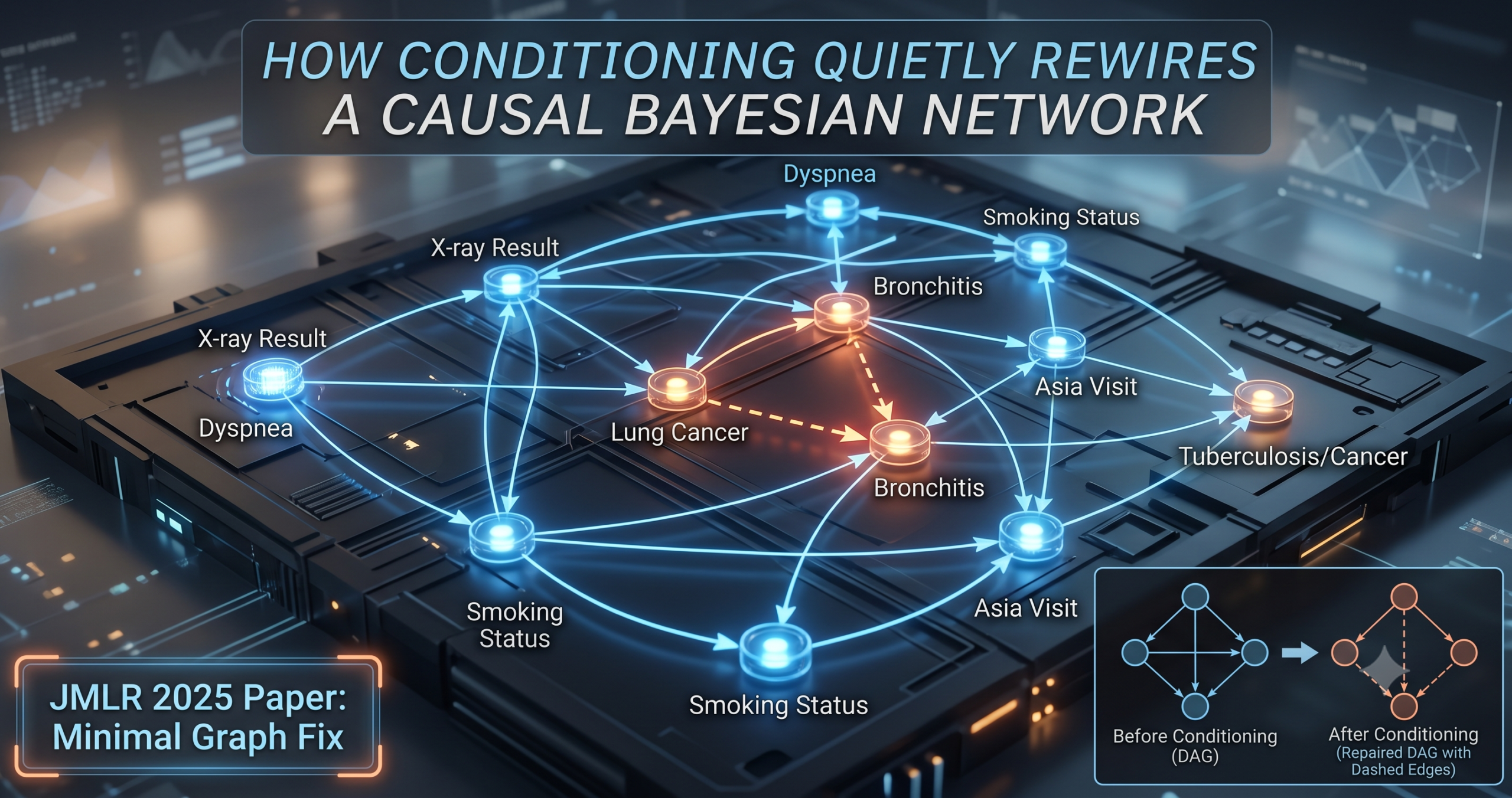
To show the repair actually matters for accuracy, not only for elegance, the authors turn to the ASIA network, the eight variable lung disease model that Lauritzen and Spiegelhalter introduced in 1988 and that has served as a teaching example ever since. The variables track recent travel to Asia, smoking status, tuberculosis, lung cancer, bronchitis, a combined indicator for tuberculosis or cancer, an X-ray result, and dyspnea, meaning shortness of breath. The conditioning set is the pair of observed symptoms, the X-ray result and dyspnea, which mirrors the realistic situation of a clinician who only sees test outcomes, not the underlying disease state directly.
The simulation compares three ways of computing the same conditional probability. The J-Method works the traditional way, building the full joint distribution with a clique tree and dividing by a normalization constant. The C-Method goes straight to the conditional distribution using the repaired minimal I map. The IC-Method, included as the naive baseline, keeps the original unmodified subgraph and pretends conditioning changed nothing structurally.
Across 100 randomly generated probability distributions, the C-Method tracked the J-Method’s results almost exactly, and that held across four entirely different topological orderings of the same graph, which is a meaningful robustness check since the repair algorithm technically depends on an arbitrary choice of order. The IC-Method told a different story. For a meaningful share of the 100 distributions its relative bias exceeded 100 percent of the true value, and for some specific cases the error reached more than 30 times the correct probability. As sample size grew from 100 to 10000 in a second experiment, both the J-Method and the C-Method showed bias and root mean square error shrinking toward zero, the signature of an unbiased estimator catching up to the truth. The IC-Method’s error stopped shrinking well before that, locked in by a structural mistake that more data simply cannot fix.
The efficiency gap is just as concrete. For the specific conditional query the authors compute by hand, the C-Method needs only 12 independent parameters against the J-Method’s 18, and it skips two of the most expensive steps in standard inference, building a clique tree and computing a normalization constant over every possible value of the remaining variables. When the authors pushed the comparison further into repeated queries with growing conditioning sets, from a single symptom variable up to seven, the clique tree approach averaged 142.860 seconds across those seven queries while the repair based approach, including the time to rerun ROS for each new conditioning set, averaged 34.596 seconds. The clique tree wins when you only ever ask about the same fixed evidence, since it reuses its one time setup cost. Once the evidence set itself starts changing, which is exactly what happens in a system fielding many different subpopulation queries, the repair approach pulls ahead.
It also works after a do-intervention
The same machinery extends to a setting that matters even more for causal claims, conditional queries after a do-intervention. Suppose a variable in the ASIA network, say tuberculosis status, is forced to a fixed level by an intervention rather than merely observed. The authors apply their method to the resulting mutilated graph, the standard causal inference move of cutting all incoming edges into the intervened variable, and then run the same closure check and repair on what is left. Estimating the interventional mean of the combined disease indicator showed the same pattern as before. The repaired graph matched the joint distribution calculation closely, while the naive approach that ignored conditioning’s effect on the mutilated graph’s structure produced errors reaching roughly 80 times the true value in some trials.
Theorem 19 in the paper gives a graphical test for which local parameters can be safely pooled across data collected under different conditioning values, the kind of question that comes up constantly when combining medical records from different hospitals or different patient cohorts, each gathered under its own selection pattern. The graph itself tells you which pieces are safe to combine and which are not, before you run a single regression.
What the authors say it cannot do
The paper is upfront about the limits of this approach, and a few are worth carrying into how you read the results. Directed acyclic graphs cannot represent feedback loops, so any system with genuine cyclic causation, common in biological and economic settings, sits outside this framework entirely. The minimal I map can also need more added edges than a more flexible graph class such as an ancestral graph or a summary graph would require, since those families have richer edge vocabularies built for exactly this purpose. The tradeoff the authors are making deliberately is to give up some of that economy in exchange for keeping the simple, computable factorization that makes a Bayesian network useful in the first place.
A second limit sits in the setup itself. The whole method assumes you already have, or have hypothesized, the full causal graph over every variable before conditioning happens. Learning that graph directly from data that has already been filtered by selection bias, with no access to the unfiltered population, remains future work by the authors’ own account, and they flag it as a promising and still largely open research direction. Finally, the benchmark networks used for the runtime tests, ASIA, Insurance, Alarm, Win95pts, Andes, and Munin, are established synthetic or semi synthetic models built for algorithm testing, not live deployments, so real world factors like streaming data quality or production latency are not part of what these numbers measure.
The conceptual shift worth remembering
Strip away the algorithm and the simulations, and the paper is making one argument that travels well beyond Bayesian networks specifically. Conditioning is not a passive act of narrowing a population. It is an operation that can actively introduce dependence structure that was not there before, and pretending otherwise is a quiet way to get confidently wrong answers from a method that looks perfectly rigorous on paper. That insight connects directly to a wider body of work on selection bias and missing data in causal graphs, including Borboudakis and Tsamardinos’s work on case control learning and Karthika Mohan, Judea Pearl, and Jin Tian’s graphical treatment of missingness, both cited in this paper’s discussion of where the idea fits into the broader field.
What sets this contribution apart from that wider literature is the choice to stay inside the DAG framework rather than jumping to a richer graph class the moment things get complicated. Keeping every original causal edge fixed, and marking the new edges as a separate, clearly non causal category, means a practitioner working in medical diagnosis or financial risk modeling does not lose the interpretability that made them choose a causal graph in the first place. The repair is additive, not a redesign.
That choice transfers naturally to other domains built on the same DAG foundation. Anywhere a causal graph is constructed once from expert knowledge and then queried repeatedly under different evidence, government policy models, financial risk systems, industrial fault diagnosis, the same closure check and the same repair algorithm apply without modification, because nothing in the method is specific to medicine beyond the worked examples chosen to explain it.
The honest remaining gap is structure learning under selection bias itself. Right now the method tells you how to fix a graph you already trust. It does not yet tell you how to build that graph from scratch when every observation you have is already filtered through the same selection process you are trying to correct for. The authors split that into a deliberate two step research program, solving the case where the full graph is known first, which is what this paper accomplishes, before tackling the harder case where it is not.
Read against that backdrop, the real contribution here is less a single algorithm and more a small, well defined piece of conceptual infrastructure. Anyone building systems that reason under selection bias now has a precise vocabulary, the C-configuration, and a fast, provably minimal way to act on it.
A working implementation of the two core algorithms
The paper’s two central procedures, the closure check and the ROS repair algorithm, are graph algorithms with no neural network involved, so the implementation below is a direct, runnable Python port rather than a deep learning model. It uses a small synthetic graph for the smoke test, built independently of the paper’s own worked examples, to keep the demonstration self contained.
Running that file prints a closure check of False and a single added edge between c and d, which matches the intuition. The collider sits at e, a direct ancestor of the conditioning variable f, and its two parents, c and d, are exactly the endpoints the algorithm flags and connects.
Closing thoughts
The achievement at the center of this paper is narrower than it might sound, and that is exactly its strength. Rather than proposing a new graph language for handling conditioning, the authors found a precise, checkable condition for when an ordinary directed acyclic graph survives conditioning unchanged, and a provably minimal way to patch it when it does not. The closure check and the ROS algorithm are both simple enough to implement in an afternoon, as the code above shows, yet they rest on a careful theoretical foundation involving terminal connecting pairs, a converging vertex sweeping operator, and several equivalent characterizations tied to Markov equivalence classes that the paper works through in full in its later sections.
The conceptual shift worth carrying forward is that conditioning is an active operation on a graph’s dependence structure, not a passive filter on rows of data. Treating it as passive, which is exactly what the IC-Method in the paper’s own simulations does, produces errors that do not shrink as you collect more data, because the mistake lives in the structure you assumed, not in the noise around an estimate. That distinction matters anywhere a system answers repeated probabilistic queries about a population defined by some observed condition, which covers far more ground than medical diagnosis alone, from financial risk scoring built on approved loan applicants to industrial monitoring built on sensor readings that only get logged past a certain threshold.
The method’s reach beyond Bayesian networks specifically comes from how little it assumes. Nothing in the closure condition or the repair algorithm depends on the variables being medical, financial, or anything else. Any causal DAG, queried repeatedly under shifting evidence, faces the same risk of picking up C-configurations, and the same fix applies without modification. That generality is what makes the contribution durable rather than a one off trick for a single application area.
The honest limitations are worth restating plainly rather than glossing over. Feedback loops are out of scope by construction, since acyclicity is load bearing for everything the paper proves. The minimal I map can need more edges than richer graph classes built specifically to minimize edge count, a tradeoff the authors accept in exchange for keeping a parameterization anyone can compute with. And the entire framework assumes the underlying causal graph is already known or hypothesized, leaving the harder problem of learning that graph directly from data already shaped by selection bias as acknowledged future work.
Where this leads next is reasonably clear from the paper’s own closing section. The authors point toward extending the same minimal I map idea to questions of causal effect estimation under selection bias, toward combining it with marginalization to study a kind of collapsibility for conditional models, and toward the harder structure learning problem itself. None of that is solved here. What is solved, carefully and with real benchmark numbers to back it up, is the first and most fundamental question. Once you condition a causal graph on evidence, exactly how much of the original structure can you still trust, and what is the smallest possible amount of new structure you need to add to trust the rest.
Frequently asked questions
What does it mean for a Bayesian network to be closed under conditioning
It means the graph you get by simply removing the conditioning variables and their edges still correctly describes the conditional independence relationships among everything left over. The paper shows this holds exactly when there are no C-configurations, meaning no collider among the ancestors of the conditioning set whose two parents are otherwise unconnected outside that set.
Why does conditioning on a variable sometimes create new dependencies between unrelated variables
This happens through a pattern statisticians call explaining away. If two causes can each independently produce the same downstream effect, learning that effect occurred, or learning facts about a descendant of that effect, makes information about one cause relevant to judging the other, even though the two causes were entirely unrelated beforehand.
What is a minimal I map and how is it different from the original causal graph
A minimal I map is the smallest graph that still correctly encodes every conditional independence relationship in a distribution, with no edge that could be removed without losing that accuracy. The paper’s minimal I map for a conditioned Bayesian network keeps every original causal edge in place and adds the fewest possible extra edges, marked as non causal, to restore that property after conditioning.
How fast is the ROS algorithm compared to standard inference
For sparse causal graphs the running time grows close to linearly with the number of ancestors of the conditioning set. In the paper’s own benchmarks it repaired a 1041 node network in under 5 seconds, and in repeated query experiments on the ASIA network it averaged roughly four times faster than the traditional clique tree approach once the conditioning set itself started changing across queries.
Can this method help combine data from different subpopulations
Yes. A theorem in the paper gives a graphical rule for which local parameters in the repaired model can be safely estimated by pooling data collected under different conditioning values, which is directly relevant to combining records from different hospitals, regions, or demographic groups that were each gathered under their own selection pattern.
Does this approach work for do-intervention queries too
It does. The authors apply the same closure check and repair to the mutilated graph that results from a do-intervention, then condition that mutilated graph on observed evidence. Their simulation on the ASIA network shows the naive approach producing errors up to roughly 80 times the true value for an interventional query, while the repaired graph again matched the gold standard calculation closely.
Go to the source
The full paper includes complete proofs, the formal terminal connecting pair characterization, and additional simulations for continuous data that were not covered here.
Xie, X., Guo, J., and Sun, Y. (2025). DAGs as Minimal I-maps for the Induced Models of Causal Bayesian Networks under Conditioning. Journal of Machine Learning Research, 26, pages 1 through 62. Editor Ilya Shpitser. Released under a CC-BY 4.0 license.
This analysis is based on the published paper and an independent evaluation of its claims.