M2OTCA Taught AI to Read Cancer Slides the Way a Pathologist Does — One Magnification at a Time
A team from Wuhan University of Science and Technology, Xiamen University, and the University of New South Wales built a multiple-magnification MIL framework that uses optimal transport to match tissue features across magnification levels, outperforming every tested baseline across four major cancer datasets while keeping computational overhead to under half a percent.
A pathologist examining a cancer biopsy does not stare at a single resolution and call it done. She zooms in to study individual cell morphology at 20x, pulls back to 10x to see how those cells organize into patterns across a tissue region, then drops to 5x to understand how the broader structure relates to the surrounding anatomy. That zoom-in-zoom-out reasoning happens naturally in expert human diagnosis. Getting a deep learning model to replicate it rather than just flattening everything into a single magnification turns out to be genuinely difficult. Zhonghang Zhu, Erik Meijering, and Liansheng Wang just published a framework that takes this challenge seriously and the numbers show it worked.
What Single-Magnification WSI Models Get Wrong
The standard approach to computational pathology has been treating whole slide image classification as a multiple instance learning problem at a single magnification level. The slide acts as a bag. Hundreds or thousands of cropped patches are the instances. A feature extractor processes each patch. An aggregation function combines those features into a single slide-level representation. A classifier makes the final call. This pipeline works remarkably well when annotated data is abundant and when the disease-relevant signal is captured at the chosen magnification.
The problem is that neither of those conditions holds reliably for histopathology. Labels are almost always at the slide level rather than the patch level, which means the model is learning from extremely weak supervision. There are no per-patch ground-truth annotations telling the model which patches actually contain cancer. The model has to figure that out for itself from thousands of unlabeled instances and a single slide-level label. This makes overfitting a persistent and serious risk.
Single magnification makes the problem worse because different magnification levels contain genuinely complementary information. High magnification at 20x captures fine cellular detail, the kind of nuclear pleomorphism and mitotic activity that pathologists use to grade malignancy. Lower magnification at 10x and 5x reveals architectural patterns, how cells are organized relative to each other and to surrounding stroma, the kinds of glandular arrangements or invasive fronts that determine subtype. When you discard two out of three magnification levels, you are discarding real diagnostic information.
Existing multi-magnification approaches have not solved this cleanly. Most of them simply train separate branches for each magnification and concatenate the outputs at prediction time. That is better than nothing, but it does not explicitly leverage the distributional consistency between magnification levels. The fact that a tissue region at 5x and the same region at 20x are describing the same underlying biology does not appear anywhere in the training signal. The model learns each magnification independently and hopes the concatenated predictions add up to something coherent.
Existing MIL methods either operate at a single magnification and discard complementary information from other levels or treat multiple magnifications as independent streams whose predictions are naively concatenated. Neither approach captures the structural consistency between magnification levels that a pathologist exploits naturally. M2OTCA addresses this by using optimal transport to explicitly align feature distributions across magnifications and gradient-based cross-attention to introduce label-derived guidance from the most informative level into the others.
The Three Innovations Inside M2OTCA
The M2OTCA framework introduces three interlinked components that together address the multi-magnification alignment problem while keeping computational costs practical for gigapixel slide processing.
Sequential Batch Prototype Formulation
Whole slide images are enormous. A single WSI at 20x magnification can contain millions of patches, making direct optimal transport computation over all instances computationally impossible. The first design decision in M2OTCA is to compress each magnification level into a compact set of regional prototypes before any cross-magnification reasoning happens.
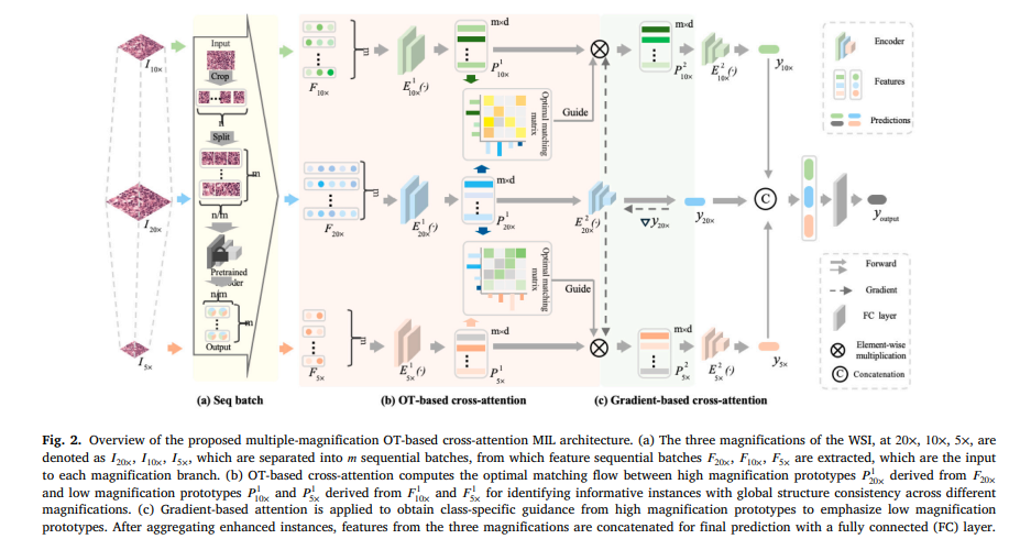
The process works like this. Given a WSI at 20x magnification, the entire image is cropped into 256×256 pixel patches ordered spatially from top left to bottom right. Those patches are divided evenly into m sequential batches. A pretrained encoder processes each patch to produce feature vectors, and those features are aggregated within each batch to produce m prototype vectors representing distinct tissue regions. The same process runs in parallel for the 10x and 5x versions of the same slide. Because patches at each magnification are split sequentially and geometrically aligned to their spatial coordinates, batch number k at 20x covers the same tissue region as batch number k at 10x and 5x. The spatial correspondence is built into the formulation rather than learned or assumed.
This prototype compression does two things at once. It reduces the optimal transport problem from aligning potentially thousands of patch features down to aligning m region-level prototypes, cutting computational complexity dramatically. And it creates representations that are genuinely comparable across magnifications because they describe the same tissue regions at different resolutions. The paper shows that 30 prototypes produces the best balance of performance and memory use across all four evaluated datasets.
Optimal Transport Based Cross-Attention
With magnification-specific prototype sets in hand, the core matching problem becomes clear. How do you identify which prototypes at 10x and 5x contain information that is relevant to the classification task, when the supervisory signal is only available at the slide level? The answer M2OTCA proposes is optimal transport based cross-attention, which uses global distributional structure rather than local pairwise similarity to guide the matching.
Optimal transport seeks the transport plan that moves probability mass from one distribution to another at minimum cost. In this context, the two distributions are the set of 20x prototypes and the set of prototypes at a lower magnification level. The cost of transporting the u-th high-magnification prototype to the v-th low-magnification prototype is the L2 distance between their feature vectors. The transport plan that minimizes total cost subject to marginal constraints is the optimal matching flow.
The key property that makes this better than attention-based matching is the marginal constraint. In standard cross-attention, each query token simply attends most strongly to whichever key tokens are most locally similar. There is no constraint on how much attention is distributed across the keys. In optimal transport matching, the marginal constraints enforce that the total mass from each source prototype is fully accounted for and that each target prototype receives exactly the mass it should based on the joint distribution. This global enforcement means a single highly distinctive high-magnification prototype cannot monopolize the matching at the expense of the rest of the slide structure. Every region has to be accounted for.
After computing the optimal transport plan between 20x and each lower magnification level, the enhanced low-magnification prototypes are computed as a transport-weighted combination of the original prototypes. The regions at 10x and 5x that correspond to the most informative high-magnification regions get upweighted. The transport plan acts as a learned filter that selects which parts of the lower-resolution views are worth attending to based on their distributional correspondence with the fine-grained 20x view.
Gradient Based Cross-Attention
The optimal transport component captures image-driven alignment, finding prototypes at different magnifications that describe the same tissue regions. The gradient-based cross-attention component adds a second complementary signal that is label-driven rather than image-driven.
The approach draws on Grad-CAM, a technique for identifying which parts of a feature representation most strongly influence a class-specific prediction. An attention-based aggregator processes the 20x prototypes and produces a slide-level prediction. The gradient of that prediction with respect to each 20x prototype is computed and global average pooled to produce a weight vector. This weight vector reflects how much each tissue region at 20x magnification contributes to the model believing this slide belongs to the target class.
Those gradient-derived weights are then used to enhance the already transport-aligned low-magnification prototypes. The enhancement is multiplicative: gradient weights from 20x scale the low-magnification prototypes so that regions of high diagnostic relevance at the fine scale are also emphasized at coarser scales. This creates a feedback loop where label information flows from the most discriminative magnification level down to the others. The result is that the 10x and 5x branches are not just geometrically aligned with 20x; they are also told which parts of the slide matter for this particular classification task.
The combined update rule for low-magnification prototypes after both cross-attention operations is compact: the enhanced 10x prototype matrix equals the transpose of the OT matching flow multiplied element-wise by the ReLU-activated gradient weights multiplied by the original 10x prototypes. The same formula applies for 5x. OT provides the structural alignment and gradient attention provides the class-discriminative emphasis, and their combination produces better-calibrated representations at every magnification level than either would achieve alone.
Standard cross-attention lets dominant prototypes monopolize the matching, ignoring distributional structure at the global level. Optimal transport enforces marginal constraints that require all mass to be transported and accounted for. On the CAMELYON16 dataset, the OT-based approach achieves 93.79 percent accuracy versus 90.47 for self-attention and 89.31 for similarity-based matching. Every competing cross-attention mechanism is statistically significantly worse at p below 0.05.
Training Objective and End-to-End Optimization
The full M2OTCA pipeline runs three magnification-specific branches in parallel during training. At the beginning of each forward pass, features extracted from the same WSI at 5x, 10x, and 20x are forwarded to their counterpart branches. Within each branch, the sequential batch encoder first compresses the patch features into m prototypes. The OT-based cross-attention then aligns low-magnification prototypes to their 20x counterparts. The gradient-based cross-attention further refines those prototypes using class-specific gradient weights derived from the 20x prediction. Each branch then generates a magnification-specific prediction from its enhanced prototypes using a second attention-based aggregator. The three predictions are concatenated and passed to a fully connected layer for the final slide-level classification output.
Training is supervised with a standard cross-entropy loss applied to the concatenated final prediction. There are no auxiliary losses, no level-specific supervision signals, and no separate training phases. The joint optimization of all encoders and the fully connected layer is end-to-end from the first batch to the last. The OT computation at each forward pass uses the Sinkhorn-Knopp algorithm to solve the discrete Kantorovich formulation efficiently, and the authors show that this adds less than 0.04 percent overhead in floating-point operations relative to a single-magnification ABMIL baseline.
The Data: Four Cancer Datasets Spanning Five Cancer Types
The evaluation covers four major public WSI benchmarks representing substantially different cancer biology and imaging characteristics.
CAMELYON16 is the breast cancer lymph node metastasis dataset with 270 training slides and 129 usable test slides after excluding one corrupt file. It is a binary classification task and one of the most widely benchmarked datasets in computational pathology. TCGA-ESCA contains 156 esophageal carcinoma slides split between squamous cell carcinoma and adenocarcinoma, a subtype classification problem with relatively limited data that tests the framework under weak supervision pressure. TCGA-Lung has 1041 slides covering lung squamous cell carcinoma and lung adenocarcinoma, the largest dataset in the evaluation set. TCGA-Kidney has 734 slides spanning three subtypes including chromophobe renal cell carcinoma, clear cell renal cell carcinoma, and papillary renal cell carcinoma, making it the only three-class problem in the benchmark.
All datasets are used at three magnification levels (5x, 10x, 20x) with patches cropped at 256×256 pixels and background patches with less than 35 percent tissue area discarded. Feature extraction uses SimCLR pretrained ResNet18 models for most settings, with an additional set of experiments using UNI foundation model features at 20x to test whether the M2OTCA cross-attention mechanisms add value on top of much stronger base encoders.
Results: Where M2OTCA Pulls Ahead
The comparison covers fifteen single-magnification methods and four multi-magnification baselines including straightforward multi-magnification extensions of CLAM and ABMIL. M2OTCA outperforms every method on every dataset in virtually all metrics, with most improvements reaching statistical significance at the paired t-test threshold of p below 0.05.
| Method | Magnification | CAMELYON16 AUC | TCGA-ESCA AUC | TCGA-Kidney AUC | TCGA-Lung AUC |
|---|---|---|---|---|---|
| ABMIL | Single (20x) | 89.10 | 84.63 | 92.77 | 91.55 |
| TransMIL | Single (20x) | 93.17 | 81.85 | 91.52 | 91.79 |
| DTFD | Single (20x) | 94.71 | 86.56 | 90.75 | 87.50 |
| CLAM_SB_3 | Multiple | 93.27 | 93.59 | 96.76 | 97.36 |
| ABMIL_3 | Multiple | 94.98 | 91.22 | 95.39 | 95.44 |
| M2OTCA (Ours) | Multiple | 96.05 | 94.21 | 97.67 | 96.49 |
Table: AUC comparison across four WSI datasets. M2OTCA achieves top AUC on three of four datasets. The TCGA-Lung AUC result (96.49) is competitive but does not reach the CLAM_SB_3 value of 97.36 on that specific metric, which the authors attribute to the dataset’s larger size and greater diversity. All other improvements are statistically significant at p below 0.05.
What the Ablation Reveals
The component-level analysis is particularly clear about what each design decision contributes. Removing all cross-attention mechanisms and simply concatenating three independent magnification branches (the M_A condition) achieves 95.19 AUC on CAMELYON16. Adding only gradient-based cross-attention (M_B) lifts this to 95.31. Adding only OT-based cross-attention (M_C) reaches 95.53. The full M2OTCA with both mechanisms achieves 96.05. Each component adds a meaningful increment and the combination exceeds either alone by a margin that is consistent across datasets.
The ablation of individual magnification levels reinforces why multi-magnification matters. The 5x branch alone on CAMELYON16 achieves only 61.86 AUC. The 10x branch alone reaches 72.48. The 20x branch reaches 94.51. Yet the full multi-magnification M2OTCA at 96.05 substantially surpasses even the strong 20x-only baseline. The gains from multi-magnification combination are real and not simply attributable to having more parameters or more training signal.
The foundation model experiment with UNI features adds another data point worth noting. When the 20x features are replaced with features from UNI, a large-scale pathology foundation model, the baseline M_A condition already achieves 97.55 AUC on TCGA-ESCA. Yet M2OTCA with UNI features still improves this to 98.98. Better base features make the cross-attention mechanisms more powerful rather than redundant, suggesting that M2OTCA is not compensating for weak feature representations but genuinely adding structural alignment value on top of strong ones.
“Our study shows that by improving the exploitation of the relationships between different magnifications and image patches using cross-magnification attention MIL mechanisms, the overfitting problem in WSI MIL can be mitigated effectively.” Zhu et al., Medical Image Analysis 2026
What the Attention Maps Show
The heat map visualizations in the paper make the model’s behavior interpretable at a level that matters clinically. For CAMELYON16 test cases with expert localization annotations, the 20x branch attention maps align closely with the manually annotated cancer regions. The model has learned to focus on the right cellular features at the right magnification without any patch-level supervision. The 10x and 5x branch maps show less precise correspondence with the annotations at those magnifications, which is exactly what the design predicts: coarser magnification levels are less precise in spatial localization but provide complementary structural context that improves classification confidence.
The failed prediction analysis is equally revealing. Cases where M2OTCA makes errors tend to involve unusually small cancerous regions, where the salient features occupy only a tiny fraction of the total slide area. At high magnification those regions contain too few patches to dominate the prototype representation, and the cross-attention mechanisms amplify signal that is structurally consistent across magnifications but spatially diffuse. This points toward a specific failure mode that future work could target with spatially aware prototype construction.
The segmentation experiment included as a generalization check is qualitatively promising. Since the model operates on patch features as inputs, the output visualization produces patch-level labels that render as coarse segments of the slide. The segmentation boundaries are jagged and imprecise compared to what a dedicated segmentation model would produce, but the regions identified as cancerous generally match expert annotations. The authors explicitly note that extending M2OTCA to fine-grained segmentation would require more specialized algorithmic design and flag this as a future research direction.
Proposed Model Code in PyTorch
The following is a complete PyTorch implementation of M2OTCA covering the full pipeline described in Sections 3.1 through 3.4 of the paper. It includes the sequential batch prototype encoder, the optimal transport based cross-attention module using the Sinkhorn-Knopp algorithm, the gradient-based cross-attention module using Grad-CAM style weights, the three-branch magnification-specific aggregators, the final concatenation classifier, and the full training loop with cross-entropy loss. A runnable smoke test on synthetic WSI data is included at the bottom.
# ============================================================
# M2OTCA: Multiple-Magnification Optimal Transport-Based
# Cross-Attention Learning for WSI Classification
# Paper: Zhu et al., Medical Image Analysis 112 (2026) 104082
# Authors: Zhonghang Zhu, Erik Meijering, Liansheng Wang
# Institutions: WUST / Xiamen University / UNSW Sydney
# ============================================================

from __future__ import annotations
import math
import torch
import torch.nn as nn
import torch.nn.functional as F
from typing import Tuple, Dict


# ─── SECTION 1: Attention-Based MIL Aggregator (AB-MIL) ───────────────────────

class ABMIL(nn.Module):
    """Attention-Based MIL aggregator (Ilse et al., 2018).

    Used as both E1(.) for prototype extraction and E2(.) for
    bag-level prediction in each magnification branch.

    For E1(.): output_dim = prototype_dim (d)  -- produces P^1 in R^{m x d}
    For E2(.): output_dim = num_classes        -- produces y prediction
    """
    def __init__(self, input_dim: int, hidden_dim: int, output_dim: int):
        super().__init__()
        self.attn_V = nn.Sequential(nn.Linear(input_dim, hidden_dim), nn.Tanh())
        self.attn_U = nn.Sequential(nn.Linear(input_dim, hidden_dim), nn.Sigmoid())
        self.attn_w = nn.Linear(hidden_dim, 1, bias=False)
        self.fc_out = nn.Linear(input_dim, output_dim)

    def forward(self, x: torch.Tensor) -> Tuple[torch.Tensor, torch.Tensor]:
        """
        Parameters
        ----------
        x : (m, D) prototype or instance features

        Returns
        -------
        out     : (output_dim,) aggregated representation or class logit
        attn_w  : (m,) attention weights for Grad-CAM computation
        """
        A = self.attn_w(self.attn_V(x) * self.attn_U(x))  # (m, 1)
        A = torch.softmax(A, dim=0).squeeze(-1)            # (m,)
        aggregated = (A.unsqueeze(-1) * x).sum(dim=0)       # (D,)
        out = self.fc_out(aggregated)
        return out, A


# ─── SECTION 2: Sequential Batch Prototype Encoder (E1) ──────────────────────

class SeqBatchEncoder(nn.Module):
    """Compress a WSI feature bag into m region structural prototypes.

    Implements Section 3.1: WSI Sequential Batch Formulation.

    Given n patch features organized in spatial order, splits them
    into m batches and applies ABMIL aggregation within each batch
    to produce m prototype vectors in R^{m x d}.

    The spatial order ensures that batch k at 20x corresponds
    geometrically to batch k at 10x and 5x, enabling the OT
    matching to align homologous tissue regions.
    """
    def __init__(self, input_dim: int, prototype_dim: int, num_prototypes: int):
        super().__init__()
        self.m = num_prototypes
        self.aggregator = ABMIL(input_dim, input_dim // 2, prototype_dim)

    def forward(self, F_bag: torch.Tensor) -> torch.Tensor:
        """
        Parameters
        ----------
        F_bag : (n, D) patch-level feature bag for one magnification

        Returns
        -------
        P1 : (m, d) region structural prototypes
        """
        n, D = F_bag.shape
        batch_size = max(1, n // self.m)
        prototypes = []
        for i in range(self.m):
            start = i * batch_size
            end = start + batch_size if i < self.m - 1 else n
            chunk = F_bag[start:end]                            # (batch_size, D)
            if chunk.shape[0] == 0:
                chunk = F_bag[-1:].clone()
            proto, _ = self.aggregator(chunk)                   # (d,)
            prototypes.append(proto)
        return torch.stack(prototypes, dim=0)                   # (m, d)


# ─── SECTION 3: Optimal Transport Cross-Attention ─────────────────────────────

class OTCrossAttention(nn.Module):
    """OT-based cross-attention to align low-magnification prototypes
    to high-magnification (20x) prototypes using Sinkhorn-Knopp.

    Implements Section 3.2: Optimal Transport-Based Cross-Attention.

    The Kantorovich formulation:
      K_{20,t}(P1_20, P1_t) = min_{O in Pi(mu_20, mu_t)}

    where C_{20,t}[u,v] = l2_dist(P1_20[u], P1_t[v])

    After solving for O_{20,t}, the enhanced prototype:
      P2_t = O_T_{20,t} @ P1_t  (transport-weighted combination)

    Sinkhorn-Knopp (1967) is used for efficient iterative solution.
    """
    def __init__(self, eps: float = 0.1, n_iters: int = 20):
        super().__init__()
        self.eps = eps
        self.n_iters = n_iters

    def sinkhorn(self, C: torch.Tensor) -> torch.Tensor:
        """Compute approximate OT plan via Sinkhorn-Knopp iterations.

        Parameters
        ----------
        C : (m, m) pairwise L2 cost matrix

        Returns
        -------
        T : (m, m) optimal transport plan with uniform marginals
        """
        m = C.shape[0]
        K = torch.exp(-C / self.eps)
        u = torch.ones(m, device=C.device) / m
        v = torch.ones(m, device=C.device) / m
        for _ in range(self.n_iters):
            u = (1.0 / m) / (K @ v + 1e-8)
            v = (1.0 / m) / (K.T @ u + 1e-8)
        T = torch.diag(u) @ K @ torch.diag(v)
        return T

    def forward(self, P1_high: torch.Tensor,
                P1_low: torch.Tensor) -> torch.Tensor:
        """
        Parameters
        ----------
        P1_high : (m, d) high-magnification (20x) prototypes
        P1_low  : (m, d) low-magnification (10x or 5x) prototypes

        Returns
        -------
        P2_low : (m, d) enhanced low-magnification prototypes
        """
        # Compute pairwise L2 cost matrix C in R^{m x m}
        C = torch.cdist(P1_high, P1_low, p=2)               # (m, m)
        C = C / (C.max() + 1e-8)                             # normalize for stability
        T = self.sinkhorn(C)                                  # (m, m) OT plan
        # Enhanced prototypes: transport-weighted combination
        P2_low = T.T @ P1_low                                  # (m, d)
        return P2_low, T


# ─── SECTION 4: Gradient-Based Cross-Attention ────────────────────────────────

def gradient_cross_attention(
    P2_ot: torch.Tensor,
    P1_high: torch.Tensor,
    pred_20x: torch.Tensor,
    target_class: int,
) -> torch.Tensor:
    """Apply Grad-CAM style weights from 20x prototypes to enhance low-mag.

    Implements Section 3.3: Gradient-Based Cross-Attention.

    Equations from the paper:
      w_c_20 = GAP(d y^c / d P1_20)      -- importance weights  (Eq. 2)
      P2_t = O_T_{20,t} x ReLU(w_c_20)^T x P1_t                 (Eq. 3-4)

    Parameters
    ----------
    P2_ot        : (m, d) OT-enhanced low-magnification prototypes
    P1_high      : (m, d) 20x prototypes (requires_grad must be True)
    pred_20x     : (num_classes,) class logit from 20x branch
    target_class : class index for gradient computation

    Returns
    -------
    P2_final : (m, d) fully enhanced low-magnification prototypes
    """
    # Compute gradient of class score w.r.t. 20x prototypes
    score = pred_20x[target_class]
    grad = torch.autograd.grad(
        score, P1_high, retain_graph=True, create_graph=False
    )[0]                                                       # (m, d)
    # Global average pooling over prototype dimension
    w_c = grad.mean(dim=-1)                                    # (m,) -- Eq. 2
    w_c_relu = F.relu(w_c).unsqueeze(-1)                      # (m, 1)
    # Element-wise weighting of OT-enhanced prototypes
    P2_final = P2_ot * w_c_relu                                  # (m, d) -- Eq. 3-4
    return P2_final


# ─── SECTION 5: M2OTCA Full Framework ─────────────────────────────────────────

class M2OTCA(nn.Module):
    """M2OTCA: Multiple-Magnification OT-based Cross-Attention MIL.

    Full framework from Section 3 and Algorithm 1 of the paper.

    Three-branch architecture:
      Branch 20x  ->  E1_20(.) -> P1_20 -> E2_20(.) -> y_20x
      Branch 10x  ->  E1_10(.) -> P1_10 -> OT(P1_20, P1_10) -> GradAttn -> P2_10
                   -> E2_10(.) -> y_10x
      Branch 5x   ->  E1_5(.)  -> P1_5  -> OT(P1_20, P1_5)  -> GradAttn -> P2_5
                   -> E2_5(.)  -> y_5x

    Final prediction: y_out = FC([y_20x; y_10x; y_5x])
    Loss: L_CE(y_out, y)

    Parameters
    ----------
    input_dim      : patch feature dimension from pretrained encoder (512)
    prototype_dim  : dimension of region prototypes d (256)
    num_prototypes : number of region prototypes m (30 in paper)
    num_classes    : number of WSI classes (2 for CAMELYON16, 3 for TCGA-Kidney)
    ot_eps         : Sinkhorn regularization (0.1)
    ot_iters       : Sinkhorn iterations (20)
    """
    def __init__(self,
                 input_dim: int = 512,
                 prototype_dim: int = 256,
                 num_prototypes: int = 30,
                 num_classes: int = 2,
                 ot_eps: float = 0.1,
                 ot_iters: int = 20):
        super().__init__()
        self.m = num_prototypes
        self.num_classes = num_classes

        # E1 encoders: feature bags -> m region prototypes at each magnification
        self.E1_20 = SeqBatchEncoder(input_dim, prototype_dim, num_prototypes)
        self.E1_10 = SeqBatchEncoder(input_dim, prototype_dim, num_prototypes)
        self.E1_5  = SeqBatchEncoder(input_dim, prototype_dim, num_prototypes)

        # E2 aggregators: enhanced prototypes -> magnification-specific predictions
        self.E2_20 = ABMIL(prototype_dim, prototype_dim // 2, num_classes)
        self.E2_10 = ABMIL(prototype_dim, prototype_dim // 2, num_classes)
        self.E2_5  = ABMIL(prototype_dim, prototype_dim // 2, num_classes)

        # OT cross-attention modules for aligning 10x and 5x to 20x
        self.ot_20_10 = OTCrossAttention(eps=ot_eps, n_iters=ot_iters)
        self.ot_20_5  = OTCrossAttention(eps=ot_eps, n_iters=ot_iters)

        # Final fully connected layer over concatenated magnification predictions
        self.fc_final = nn.Linear(num_classes * 3, num_classes)

    def forward(self,
                F_20: torch.Tensor,
                F_10: torch.Tensor,
                F_5:  torch.Tensor,
                target_class: int = 0) -> Dict:
        """
        Full M2OTCA forward pass following Algorithm 1.

        Parameters
        ----------
        F_20  : (n_20, D) patch features at 20x magnification
        F_10  : (n_10, D) patch features at 10x magnification
        F_5   : (n_5,  D) patch features at 5x magnification
        target_class : class index used for gradient-based cross-attention

        Returns
        -------
        dict with logits, branch predictions, prototypes, and OT plans
        """
        # ── Step 1: Compute region structural prototypes (SeqBatch) ──────────
        P1_20 = self.E1_20(F_20)                               # (m, d)
        P1_10 = self.E1_10(F_10)                               # (m, d)
        P1_5  = self.E1_5(F_5)                                 # (m, d)

        # Enable grad on P1_20 for Grad-CAM weight computation
        P1_20.requires_grad_(True)

        # ── Step 2: 20x branch prediction (used for gradient computation) ────
        pred_20x, attn_20 = self.E2_20(P1_20)                  # (num_classes,), (m,)

        # ── Step 3: OT-based cross-attention to align 10x and 5x to 20x ─────
        P2_10_ot, T_20_10 = self.ot_20_10(P1_20.detach(), P1_10)  # (m, d)
        P2_5_ot,  T_20_5  = self.ot_20_5(P1_20.detach(), P1_5)    # (m, d)

        # ── Step 4: Gradient-based cross-attention (Eq. 2-4 in paper) ─────────
        P2_10 = gradient_cross_attention(P2_10_ot, P1_20, pred_20x, target_class)
        P2_5  = gradient_cross_attention(P2_5_ot,  P1_20, pred_20x, target_class)

        # ── Step 5: Low-magnification branch predictions ───────────────────────
        pred_10x, attn_10 = self.E2_10(P2_10.detach())          # (num_classes,)
        pred_5x,  attn_5  = self.E2_5(P2_5.detach())            # (num_classes,)

        # ── Step 6: Concatenate all magnification predictions + FC layer ───────
        combined = torch.cat([pred_20x, pred_10x, pred_5x], dim=0)  # (3 * C,)
        y_out = self.fc_final(combined)                             # (num_classes,)

        return {
            'logits':    y_out,
            'y_20x':     pred_20x,
            'y_10x':     pred_10x,
            'y_5x':      pred_5x,
            'P1_20':     P1_20,
            'P1_10':     P1_10,
            'P2_10':     P2_10,
            'T_20_10':   T_20_10,
            'T_20_5':    T_20_5,
            'attn_20':   attn_20,
        }


# ─── SECTION 6: Training Loss ─────────────────────────────────────────────────

def m2otca_loss(logits: torch.Tensor, label: torch.Tensor) -> torch.Tensor:
    """Cross-entropy training loss (Equation 5 in paper).

    The loss is applied to the final concatenated prediction y_out.
    No auxiliary per-magnification losses are used during training.
    All three magnification branches are jointly optimized through
    this single slide-level supervision signal.
    """
    return F.cross_entropy(logits.unsqueeze(0), label.unsqueeze(0))


# ─── SECTION 7: Smoke Test ─────────────────────────────────────────────────────

def _smoke_test():
    """End-to-end smoke test of M2OTCA on synthetic WSI patch features.

    Verifies:
      - Forward pass through full three-branch architecture
      - OT matching between high and low magnification prototypes
      - Gradient-based cross-attention weight computation
      - Loss computation and backward pass through all components
    """
    print("=" * 60)
    print("M2OTCA Smoke Test -- Synthetic WSI Patch Features")
    print("Paper: Zhu et al., Medical Image Analysis 112 (2026) 104082")
    print("=" * 60)

    device = 'cuda' if torch.cuda.is_available() else 'cpu'
    print(f"\nDevice: {device}")

    # Synthetic patch features -- reduced sizes for fast testing
    n_20, n_10, n_5 = 300, 75, 20    # approximate ratio: 4:1 between adjacent levels
    input_dim = 512                    # SimCLR ResNet18 feature dimension
    prototype_dim = 256                # d in paper
    num_prototypes = 30                # m in paper (best value from ablation)
    num_classes = 2                    # binary (cancer vs normal, CAMELYON16)

    F_20 = torch.randn(n_20, input_dim, device=device)
    F_10 = torch.randn(n_10, input_dim, device=device)
    F_5  = torch.randn(n_5,  input_dim, device=device)
    label = torch.tensor(1, device=device)  # ground truth: cancer

    model = M2OTCA(
        input_dim=input_dim,
        prototype_dim=prototype_dim,
        num_prototypes=num_prototypes,
        num_classes=num_classes,
        ot_eps=0.1,
        ot_iters=20,
    ).to(device)
    model.train()

    total_params = sum(p.numel() for p in model.parameters())
    print(ff"Total parameters: {total_params:,}")
    print(ff"Patch counts: 20x={n_20}  10x={n_10}  5x={n_5}")
    print(ff"Prototypes m={num_prototypes}  Prototype dim d={prototype_dim}")

    optimizer = torch.optim.Adam(model.parameters(), lr=1e-3, weight_decay=1e-4)

    # Forward pass
    out = model(F_20, F_10, F_5, target_class=label.item())

    # Compute and backprop training loss
    loss = m2otca_loss(out['logits'], label)
    optimizer.zero_grad()
    loss.backward()
    optimizer.step()

    print(ff"\n{'─'*40}")
    print(ff"Training loss:     {loss.item():.4f}")
    print(ff"Final logit shape: {list(out['logits'].shape)}")
    print(ff"Prototype P1_20:   {list(out['P1_20'].shape)}")
    print(ff"OT plan T_20_10:   {list(out['T_20_10'].shape)}")
    print(ff"Enhanced P2_10:    {list(out['P2_10'].shape)}")
    print(ff"Pred y_20x:        {out['y_20x'].detach().cpu().numpy().round(3)}")
    print(ff"Pred y_10x:        {out['y_10x'].detach().cpu().numpy().round(3)}")
    print(ff"Pred y_5x:         {out['y_5x'].detach().cpu().numpy().round(3)}")
    print(f"{'─'*40}")

    # Inference mode (no gradient tracking needed)
    model.eval()
    with torch.no_grad():
        out_inf = model(F_20, F_10, F_5, target_class=0)
    probs = torch.softmax(out_inf['logits'], dim=0)
    print(ff"\nInference cancer probability: {probs[1].item():.3f}")
    print("Smoke test passed. M2OTCA forward and backward cycles OK.")
    print("See Algorithm 1 in Zhu et al. 2026 for the full training workflow.")
    print("=" * 60)


if __name__ == '__main__':
    _smoke_test()
What M2OTCA Opens Up and Where the Gaps Remain
The cross-dataset generalization results across four entirely different cancer types and tissue preparations demonstrate something meaningful about the approach. A model trained on lymph node tissue for CAMELYON16, esophageal tissue for TCGA-ESCA, lung parenchyma for TCGA-Lung, and kidney cortex for TCGA-Kidney does not share a common visual vocabulary between datasets. The fact that M2OTCA consistently outperforms competing methods across all of these suggests that the OT alignment and gradient-based enhancement are capturing structure that is genuinely useful across diverse histological contexts and not specific to any one tissue type.
The computational overhead analysis is reassuring for practical deployment. The OT computation adds only 0.04 percent overhead in FLOPs relative to the ABMIL baseline. The multi-magnification setting as a whole increases FLOPs by approximately 24 percent compared to processing a single magnification, which is modest given that it provides three complete views of the tissue at different scales. The prototype compression step is what makes this practical. Without compressing WSI patches into m regional prototypes first, the OT computation over thousands of raw patch features would be prohibitively expensive.
There are genuine limitations worth acknowledging. The only case where M2OTCA falls short is AUC on TCGA-Lung, where the multi-magnification CLAM_SB_3 baseline achieves 97.36 versus M2OTCA’s 96.49. The authors suggest this may relate to the dataset’s larger size and greater diversity making the cross-magnification alignment less consistently beneficial when there is sufficient data for single-magnification methods to learn strong representations independently. This points toward a question about when multi-magnification alignment is most valuable and when large datasets and strong encoders can compensate for the absence of cross-scale reasoning.
The failed prediction analysis flags a specific weakness around small lesion detection. When cancerous regions are spatially concentrated in a tiny fraction of the total slide area, the prototype representation dilutes their signal because most prototypes correspond to healthy tissue. A more spatially adaptive prototype construction that oversamples regions flagged as potentially informative at high magnification could address this directly. The paper notes this as a future direction.
The authors explicitly identify several promising extensions. Intra-magnification feature distribution alignment using OT-based loss functions could improve interpretability at each individual magnification level rather than only across magnifications. The optimization direction for cross-magnification guidance could be made adaptive, deriving guidance from whichever magnification level is most informative for a given slide rather than always flowing from high to low magnification. Extension beyond classification to segmentation and localization would require finer-grained algorithmic design but would substantially increase clinical utility. And the framework is not inherently limited to three magnification levels; the OT-based alignment mechanism extends naturally to more levels, which is relevant for scanners that capture additional intermediate resolutions.
The broader point is about what structural assumptions we build into medical AI. M2OTCA encodes a specific claim about how diagnostic information is organized in histopathology slides: that different magnification levels contain complementary information, that the distributions of tissue features across those levels are structurally consistent in ways that can be aligned globally rather than locally, and that label-derived importance weights from the most discriminative magnification should guide representation learning at coarser scales. That claim is grounded in decades of pathology practice, and the results across four cancer types and thousands of slides suggest it is correct. That is a more satisfying foundation for a diagnostic AI system than a flat feature aggregator that treats the problem as an unstructured pattern recognition task without any prior knowledge about how the biology is organized.
Read the Full Paper
The complete M2OTCA paper with full experimental details, ablation studies across all four datasets, and heat map visualizations is available open access via ScienceDirect.
Zhu, Z., Meijering, E., & Wang, L. (2026). M2OTCA: Multiple-magnification optimal transport-based cross-attention learning for whole slide image classification. Medical Image Analysis, 112, 104082. https://doi.org/10.1016/j.media.2026.104082
This article is an independent editorial analysis of peer-reviewed research. The PyTorch implementation is an educational reproduction and may differ from any official repository in engineering details. For research use, verify against the original paper. This work was supported by the National Natural Science Foundation of China (Grant No. 62371409) and the China Scholarship Council (CSC).