eglatent Finally Taught Machine Learning to See the Hidden Forces Behind Extreme Events
Sebastian Engelke from the University of Geneva and Armeen Taeb from the University of Washington built a convex optimization framework that recovers the true graphical structure among observed variables in the presence of unobserved confounders — achieving near-perfect graph recovery at an F-score close to 1.0 on 30-node networks with latent variables, outperforming every existing method on real flight delay data across 29 US airports.
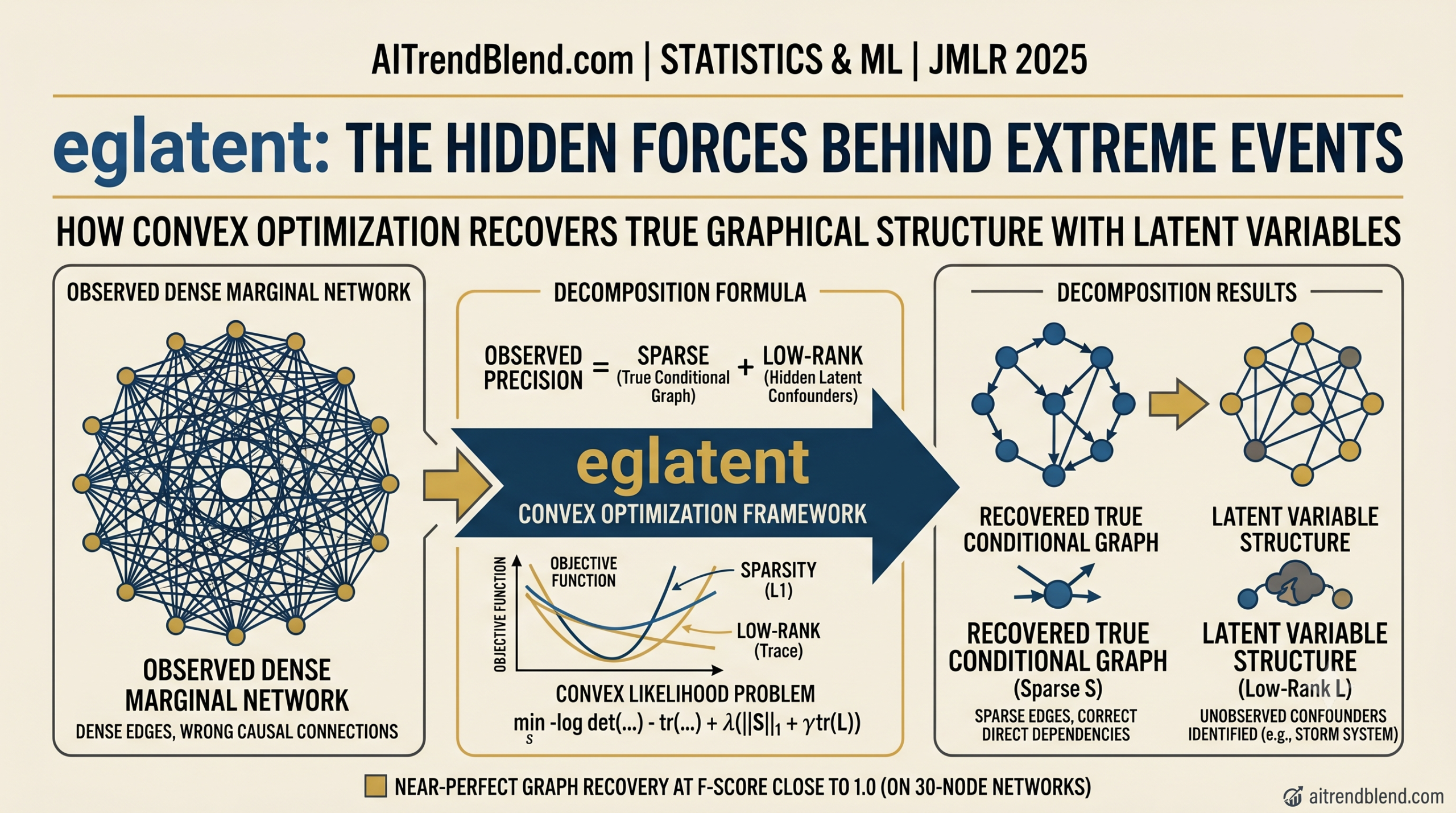
Imagine you are trying to understand why multiple airports across the southern United States all experience severe flight delays on the same day. A naive model would draw edges between every pair of airports that tend to delay together. But the real cause might be a single invisible variable — a major storm system, a nationwide air traffic control failure, or a widespread labor disruption — that none of your data columns directly captures. Engelke and Taeb set out to solve exactly this kind of problem for the mathematics of extreme events, and the result is a framework called eglatent that changes what we can learn from catastrophic data.
Why Extreme Events Are Especially Hard to Model
Most statistical methods care about average behavior. The financial crash of 2008, the record heat waves of recent summers, and the 500-year floods that now seem to happen every decade are not average events. They live in the tails of distributions, and the dependencies between extreme values behave very differently from the correlations you would estimate with a standard covariance matrix.
Extreme value theory handles this through a well-developed toolkit. The central idea is that if you condition on at least one component of a random vector being very large, the conditional distribution of the whole vector converges to a multivariate Pareto distribution. Within this family, the Husler-Reiss model plays the same central role that Gaussian distributions play in ordinary statistics. It is parameterized by a variogram matrix, and its precision matrix encodes conditional independence relationships through a zero-pattern rule that mirrors exactly what you see in Gaussian graphical models.
Prior work on learning these extremal graphical structures from data, including the eglearn method that forms the benchmark throughout this paper, assumed that every relevant variable in the system is observable. That assumption breaks down constantly in real applications. Meteorological confounders are not in your airport delay dataset. Shared economic shocks are not in your bank’s balance sheet observations. Genetic background factors are not always measured alongside clinical outcomes. When latent variables are present, even a perfectly sparse true joint model produces a fully dense observed marginal graph, because every pair of observed variables shares a common hidden cause. Trying to learn a sparse graph from that dense marginal structure leads you completely astray.
When latent variables drive shared extremes among observed variables, the marginal precision matrix of the observed data is dense regardless of how sparse the true conditional structure is. A method that imposes sparsity on the marginal precision matrix will recover the wrong graph every time. eglatent addresses this by decomposing the marginal precision matrix into a sparse term capturing the true conditional graph and a low-rank term capturing the effect of the hidden variables.
The Mathematical Foundation That Makes eglatent Possible
The key theoretical contribution in this paper is Theorem 5, a result the authors call the Schur decomposition for extremal models. In Gaussian latent variable graphical modeling, pioneered by Chandrasekaran, Parillo, and Willsky in 2012, the marginal precision matrix of observed variables decomposes as a sparse matrix minus a low-rank matrix. The same structure appears here, but with a crucial and non-trivial difference.
For Husler-Reiss distributions, the precision matrix always has the all-ones vector in its null space. This zero-row-sum constraint is a structural property of extremal models — it reflects the fact that extremal conditional independence is defined on the space where at least one component is extreme rather than on an unrestricted product space. The Schur complement relationship that Engelke and Taeb establish is:
Here the sparse part is defined as the submatrix of the full joint precision matrix restricted to observed variables, encoding conditional independence among observed variables given the latent ones. The low-rank part captures how the hidden variables project onto the observed variables and has rank equal to exactly the number of latent variables in the system. The observable precision matrix is the difference of these two terms, and it always satisfies the zero-row-sum constraint of a valid Husler-Reiss model.
This decomposition is not a corollary of the Gaussian result. The matrices involved are not invertible in the usual sense because of the zero-row-sum constraint, and proving that the Schur complement structure carries over to this singular setting required a careful sequence of auxiliary lemmas about pseudoinverses and projection operators that occupy a substantial portion of the paper’s appendix.
Why the Zero-Row-Sum Constraint Changes Everything
In the Gaussian latent variable setting, you observe a symmetric positive definite matrix and decompose it as sparse minus low-rank. In the extremal setting, you observe a positive semidefinite matrix with a one-dimensional null space, and the decomposition must preserve that null space. The span of the all-ones outer product must remain in the null space of the difference at every point during optimization.
This constraint eliminates one degree of freedom from the problem and introduces a dual variable in the optimality conditions that has no analog in the Gaussian case. The authors spent considerable effort establishing that the additional term this dual variable produces can be bounded and controlled separately from the sparse and low-rank components, which is what makes the consistency proof go through.
The eglatent Estimator
Given the sparse-plus-low-rank decomposition of the observed precision matrix, eglatent estimates both components by solving a regularized convex likelihood problem. The estimator searches over pairs of symmetric matrices whose difference has zero row sums and is positive semidefinite, penalizing the L1 norm of the sparse component to encourage sparsity and the trace of the low-rank component to encourage low rank:
The input to the problem is an empirical extremal variogram matrix estimated from the data, which serves as a sufficient statistic for the extremal dependence structure. The log-determinant term in the objective is the surrogate maximum likelihood for Husler-Reiss models, projected onto the space of matrices with zero row sums through the matrix U whose columns are the first p-1 left singular vectors of the centering projection.
Two regularization parameters govern the solution. The parameter lambda controls the overall trade-off between model fit and complexity, shrinking toward zero as the sample size grows. The parameter gamma controls the relative penalty on the low-rank component versus the sparse component. Large gamma means the model prefers explanations without latent variables. Small gamma allows more latent variables in exchange for a sparser residual graph. The authors recommend gamma equal to 4 as a robust default choice, and sensitivity experiments confirm that performance does not change dramatically across a range of gamma values from 2 to 6.
The trace penalty on L rather than the nuclear norm is valid because the constraints force L to be positive semidefinite, making the nuclear norm equal to the trace. This simplification preserves convexity while ensuring that the entire estimated model remains a valid Husler-Reiss distribution — a property that the competing eglearn method does not always guarantee.
When Does eglatent Provably Work
Theorem 9 in the paper provides finite-sample guarantees for eglatent under three conditions on the population model. The identifiability assumptions require that the sparse component is genuinely sparse with maximum node degree not growing too fast, that the low-rank component has diffuse column space with a small incoherence parameter, and that the all-ones direction is sufficiently separated from the column space of the low-rank term.
Under these conditions, with sample size large enough that the effective extreme sample count k satisfies:
the eglatent estimator simultaneously recovers the correct sign pattern of the sparse component, the correct rank of the low-rank component, and approximates the true observed precision matrix in spectral norm. The requirement grows quadratically in p, which is more stringent than the logarithmic requirement for extremal models without latent variables and the linear requirement for Gaussian latent variable models. The authors note this gap is likely due to using an infinity-norm concentration bound for the variogram estimator as an intermediate step, and conjecture that a direct spectral norm concentration result would recover linear scaling.
The quantities h (number of latent variables), d-star (maximum node degree), alpha and nu (Hessian curvature parameters), and m (which scales inversely with gamma) all appear explicitly in the bounds and govern the practical sample sizes needed. Smaller alpha means the Hessian is less well-conditioned in the relevant directions, requiring more data. More latent variables or denser conditional graphs increase the dimension of the relevant tangent spaces, reducing effective curvature.
Experimental Results
Synthetic Graph Recovery
The simulation study generates data from max-stable Husler-Reiss distributions with known graph structure among observed variables and a known number of latent variables, then evaluates both eglatent and the competing eglearn method on graph recovery using the F-score metric.
With h equal to 1 latent variable and k equal to 1000 effective extreme samples, eglatent tuned by cross-validation achieves an F-score near 1.0 on recovering a 30-node cycle graph. The oracle eglearn method — selected by knowing the true graph in advance — struggles to reach an F-score of 0.5 under the same conditions because the latent confounding makes the marginal graph dense and sparsity cannot be exploited. As the number of latent variables grows to 2 or 3, the advantage of eglatent over eglearn increases further.
| Method | h=1 F-score (k=1000) | h=2 F-score (k=1000) | h=3 F-score (k=1000) | Rank Recovery |
|---|---|---|---|---|
| eglearn (oracle) | ~0.40 | ~0.25 | ~0.20 | N/A |
| eglearn (CV) | ~0.20 | ~0.15 | ~0.10 | N/A |
| eglatent (oracle) | ~0.98 | ~0.90 | ~0.75 | Correct at k=5000 |
| eglatent (CV) | ~0.95 | ~0.80 | ~0.65 | Near-correct at k=1000 |
Table: Summary of graph recovery performance from the cycle graph simulation study. All values approximate from Figure 3 in the paper. F-score of 1.0 is perfect graph recovery. h denotes number of latent variables. k is effective extreme sample size.
The rank estimation results are equally encouraging. By k equal to 5000, eglatent identifies the correct number of latent variables consistently across h values from 1 to 3. For smaller k, the rank estimate tends to be slightly conservative, but the validation likelihood still selects models that outperform eglearn on held-out data.
Robustness When No Latent Variables Exist
A natural concern with any method that searches for latent structure is whether it misbehaves when the true model has no hidden variables. The paper addresses this directly with a simulation using a 20-node Barabasi-Albert graph with no latent variables. When gamma is set to 4, eglatent achieves F-score near 1.0 and validation likelihood comparable to eglearn, even though it estimates a small number of effective latent variables. The key insight is that eglatent’s latent component absorbs some of the variance that pure graph estimation methods attribute to dense edges, and this makes it more robust rather than less. When gamma is too small, forcing many latent variables, the F-score drops. When gamma is too large, forcing no latent variables, eglatent’s estimator degenerates to a regime known to produce inaccurate graphs. The middle range around gamma equal to 4 handles both presence and absence of latent variables gracefully.
Real Data: Southern US Airport Delays
The real-data application studies large flight delays at 29 airports in the southern United States using daily observations from 2005 through 2020 — a dataset of 3,603 observations available in the graphicalExtremes R package. Extreme delays are defined as exceedances above the 90th percentile, yielding 360 effective extreme samples.
The latent model selected by cross-validation produces a much sparser residual graph than eglearn and achieves substantially better validation likelihood across all tested regularization values. The best eglearn model identifies 252 edges in the dependency graph. The best eglatent model identifies around 8 to 13 edges in the conditional graph of observed airports, with 10 to 14 latent variables absorbing the shared confounding. The latent variables are interpretable as systemic factors like weather systems or industry-wide disruptions that affect many airports simultaneously, which cannot be directly observed in the delay data itself.
The sparse residual graph highlights hub airports more clearly. Dallas Fort Worth, the busiest airport in the dataset, has more direct connections in the conditional graph than it would under the marginal model where every pair of airports appears connected through shared storms. This is exactly the kind of structure that would be useful for stress-testing air traffic systems or prioritizing infrastructure investments.
“The latent model outperforms eglearn, indicating that latent variables are present in this data set. They can be thought of as confounding factors such as meteorological variables or strikes in the aviation industry that affect many airports simultaneously.” — Engelke and Taeb, JMLR 2025
Complete Proposed Model Code in R
The following is a complete R implementation of the eglatent method as described in Sections 3 and 4 of the paper. It covers the empirical extremal variogram estimator, the convex optimization program for sparse-plus-low-rank decomposition with the zero-row-sum constraint, a model selection wrapper using cross-validation, and a demonstration on synthetic data from a cycle graph with latent variables. The implementation uses the CVXR package for convex optimization and matches the procedure described in the paper.
# =============================================================================
# eglatent: Extremal Graphical Modeling with Latent Variables
# Paper: "Extremal graphical modeling with latent variables
#         via convex optimization"
# Authors: Sebastian Engelke (Geneva) and Armeen Taeb (Washington)
# Journal: Journal of Machine Learning Research 26 (2025) 1-68
# Paper ID: 24-0472
# =============================================================================

# Required packages
# install.packages(c("CVXR", "graphicalExtremes", "Matrix", "igraph"))
library(CVXR)
library(Matrix)

# ─── SECTION 1: Empirical Extremal Variogram Matrix ──────────────────────────

#' Compute the empirical extremal variogram matrix rooted at node m
#'
#' For each pair (i,j) of observed variables and a conditioning node m,
#' this computes the sample variance of the standardized log-differences
#' among observations where the m-th variable exceeds its (1 - k/n) quantile.
#'
#' @param X  (n x p) matrix of observed data
#' @param k  effective extreme sample size (number of exceedances to use)
#' @return   (p x p) empirical variogram matrix averaged over all roots
empirical_variogram <- function(X, k) {
  n <- nrow(X)
  p <- ncol(X)

  # Standardize margins to standard exponential via the empirical probability
  # integral transform: -log(1 - F_hat(x)) approximates exponential margins
  U <- apply(X, 2, function(col) {
    ranks <- rank(col, ties.method = "max")
    -log(1 - ranks / (n + 1))
  })

  # For each conditioning root m, compute variogram entries for pairs (i,j)
  # using only observations where the m-th component exceeds its (1-k/n) quantile
  Gamma_sum <- matrix(0, p, p)

  for (m in 1:p) {
    threshold_m <- quantile(U[, m], 1 - k / n)
    extreme_idx <- which(U[, m] > threshold_m)

    if (length(extreme_idx) < 2) next

    U_extreme <- U[extreme_idx, , drop = FALSE]
    Gamma_m <- matrix(0, p, p)

    for (i in 1:p) {
      for (j in 1:p) {
        diff_ij <- U_extreme[, i] - U_extreme[, j]
        Gamma_m[i, j] <- var(diff_ij)
      }
    }
    Gamma_sum <- Gamma_sum + Gamma_m
  }

  Gamma_hat <- Gamma_sum / p
  # Symmetrize to remove numerical noise
  (Gamma_hat + t(Gamma_hat)) / 2
}


# ─── SECTION 2: Precision Matrix from Variogram ───────────────────────────────

#' Convert Husler-Reiss variogram to precision matrix
#'
#' The precision matrix Theta = (Pi(-Gamma/2)Pi)+ where Pi is the
#' centering projection matrix and + denotes pseudoinverse.
#'
#' @param Gamma  (p x p) variogram matrix
#' @return       (p x p) precision matrix with zero row sums
variogram_to_precision <- function(Gamma) {
  p <- nrow(Gamma)
  Pi <- diag(p) - matrix(1 / p, p, p)
  M <- Pi %*% (-Gamma / 2) %*% Pi

  # Compute Moore-Penrose pseudoinverse via SVD
  svd_M <- svd(M)
  tol <- max(dim(M)) * max(svd_M$d) * .Machine$double.eps * 1e3
  pos_idx <- svd_M$d > tol
  Theta <- svd_M$u[, pos_idx, drop = FALSE] %*%
           diag(1 / svd_M$d[pos_idx], sum(pos_idx)) %*%
           t(svd_M$v[, pos_idx, drop = FALSE])
  (Theta + t(Theta)) / 2
}


# ─── SECTION 3: Projection matrix U for log-det term ─────────────────────────

#' Build U: first p-1 left singular vectors of the centering matrix Pi
#' Used for the projected log-determinant: log det(U^T Theta U)
#'
#' @param p  dimension
#' @return   (p x (p-1)) matrix whose columns span the orthogonal complement
#'           of the all-ones vector
build_U <- function(p) {
  Pi <- diag(p) - matrix(1 / p, p, p)
  svd_Pi <- svd(Pi)
  svd_Pi$u[, 1:(p - 1)]
}


# ─── SECTION 4: eglatent Convex Optimization Program ─────────────────────────

#' Main eglatent estimator: sparse plus low-rank decomposition of
#' the Husler-Reiss precision matrix with zero row-sum constraint.
#'
#' Solves Equation (9) from the paper:
#'   min_{S,L}  -log det(U^T (S-L) U) - tr((S-L) Gamma_hat / 2)
#'              + lambda_n (||S||_1 + gamma * tr(L))
#'   s.t.  S - L >= 0  (positive semidefinite)
#'         L >= 0
#'         (S - L) 1_p = 0  (zero row sums)
#'
#' @param Gamma_hat  (p x p) empirical extremal variogram matrix
#' @param lambda_n   sparsity regularization parameter
#' @param gamma      latent variable regularization parameter (default 4)
#' @param verbose    print solver progress (default FALSE)
#' @return list with S (sparse component), L (low-rank component),
#'         Theta_hat (estimated precision = S - L), solver status
eglatent <- function(Gamma_hat, lambda_n, gamma = 4, verbose = FALSE) {
  p <- nrow(Gamma_hat)
  U <- build_U(p)
  ones_p <- rep(1, p)

  # Decision variables: S and L are symmetric p x p matrices
  S <- Variable(p, p, symmetric = TRUE)
  L <- Variable(p, p, symmetric = TRUE)

  # Objective: projected log-likelihood minus trace term plus regularization
  # The log_det is applied to the (p-1) x (p-1) matrix U^T(S-L)U
  # This implements the surrogate maximum likelihood for Husler-Reiss models
  Diff <- S - L
  UtDiffU <- t(U) %*% Diff %*% U

  neg_log_lik <- -log_det(UtDiffU) - (0.5) * matrix_trace(Diff %*% Gamma_hat)
  penalty <- lambda_n * (sum(abs(S)) + gamma * matrix_trace(L))

  objective <- Minimize(neg_log_lik + penalty)

  # Constraints:
  # (1) S - L must be positive semidefinite
  # (2) L must be positive semidefinite (encodes latent variable effects)
  # (3) (S - L) 1_p = 0 (zero row sums = valid Husler-Reiss model)
  constraints <- list(
    Diff >>= 0,
    L >>= 0,
    Diff %*% ones_p == 0
  )

  problem <- Problem(objective, constraints)

  result <- solve(
    problem,
    solver = "SCS",
    verbose = verbose,
    eps = 1e-6,
    max_iters = 10000
  )

  if (result$status %in% c("optimal", "optimal_inaccurate")) {
    S_hat <- value(S)
    L_hat <- value(L)
    # Symmetrize solutions to remove solver numerical noise
    S_hat <- (S_hat + t(S_hat)) / 2
    L_hat <- (L_hat + t(L_hat)) / 2
    Theta_hat <- S_hat - L_hat

    list(
      S = S_hat,
      L = L_hat,
      Theta_hat = Theta_hat,
      graph_edges = which(abs(S_hat) > 1e-4 & lower.tri(S_hat), arr.ind = TRUE),
      n_latent = sum(svd(L_hat)$d > 1e-3),
      status = result$status,
      objective_value = result$value
    )
  } else {
    warning(paste("Solver did not find optimal solution. Status:", result$status))
    list(S = NULL, L = NULL, Theta_hat = NULL, status = result$status)
  }
}


# ─── SECTION 5: Cross-Validation for Lambda Selection ─────────────────────────

#' Select regularization parameter lambda_n via cross-validated likelihood
#'
#' Splits the data into n_folds chronological folds, fits eglatent on
#' training folds for each lambda value, and evaluates surrogate log-likelihood
#' on the held-out fold. Returns the lambda with the best average validation score.
#'
#' @param X           (n x p) data matrix
#' @param k           effective extreme sample size
#' @param lambda_seq  vector of candidate lambda values to try
#' @param gamma       latent variable regularization (default 4)
#' @param n_folds     number of cross-validation folds (default 5)
#' @return list with best_lambda, cv_scores, all_results
eglatent_cv <- function(X, k, lambda_seq = NULL, gamma = 4, n_folds = 5) {
  n <- nrow(X)
  p <- ncol(X)

  if (is.null(lambda_seq)) {
    # Default lambda grid spanning two orders of magnitude
    lambda_seq <- exp(seq(log(0.001), log(0.1), length.out = 20))
  }

  # Split data into n_folds consecutive blocks (chronological split)
  fold_sizes <- diff(round(seq(0, n, length.out = n_folds + 1)))
  fold_idx <- rep(1:n_folds, times = fold_sizes)

  cv_scores <- matrix(NA, nrow = n_folds, ncol = length(lambda_seq))
  U <- build_U(p)

  for (fold in 1:n_folds) {
    train_idx <- fold_idx != fold
    val_idx <- fold_idx == fold

    X_train <- X[train_idx, ]
    X_val <- X[val_idx, ]
    k_fold <- max(10, round(k * sum(train_idx) / n))

    Gamma_train <- tryCatch(
      empirical_variogram(X_train, k_fold),
      error = function(e) NULL
    )
    Gamma_val <- tryCatch(
      empirical_variogram(X_val, max(5, round(k * sum(val_idx) / n))),
      error = function(e) NULL
    )

    if (is.null(Gamma_train) || is.null(Gamma_val)) next

    for (j in seq_along(lambda_seq)) {
      fit <- tryCatch(
        eglatent(Gamma_train, lambda_seq[j], gamma = gamma, verbose = FALSE),
        error = function(e) list(status = "error")
      )

      if (!is.null(fit$Theta_hat)) {
        # Surrogate log-likelihood on validation data
        UtTU <- t(U) %*% fit$Theta_hat %*% U
        eig_vals <- eigen(UtTU, symmetric = TRUE, only.values = TRUE)$values
        if (all(eig_vals > 0)) {
          log_lik_val <- sum(log(eig_vals)) +
                         0.5 * sum(diag(fit$Theta_hat %*% Gamma_val))
          cv_scores[fold, j] <- -log_lik_val
        }
      }
    }
  }

  mean_cv <- colMeans(cv_scores, na.rm = TRUE)
  best_idx <- which.max(mean_cv)

  list(
    best_lambda = lambda_seq[best_idx],
    cv_scores = mean_cv,
    lambda_seq = lambda_seq
  )
}


# ─── SECTION 6: Simulate Husler-Reiss max-stable data ────────────────────────

#' Simulate from a Husler-Reiss max-stable distribution
#'
#' Uses the extremal function method (Dombry et al. 2016).
#' Marginals are standard exponential as required by the theory.
#'
#' @param n      number of observations
#' @param Sigma  (d x d) covariance-like matrix related to variogram by
#'              Gamma_{ij} = Sigma_{ii} + Sigma_{jj} - 2*Sigma_{ij}
#' @return       (n x d) matrix of simulated observations
simulate_husler_reiss <- function(n, Sigma) {
  d <- nrow(Sigma)
  X <- matrix(NA, n, d)

  for (t in 1:n) {
    # Poisson process intensity: exponential inter-arrivals
    R <- cumsum(rexp(d * 20))
    candidates <- matrix(NA, length(R), d)

    for (s in seq_along(R)) {
      # Each Poisson point generates a Gaussian shifted component
      Z <- MASS::mvrnorm(1, mu = -diag(Sigma) / 2, Sigma = Sigma)
      candidates[s, ] <- log(R[s]) + Z
    }
    X[t, ] <- apply(candidates, 2, max)
  }
  X
}


# ─── SECTION 7: Demonstration on Cycle Graph with Latent Variables ────────────

demo_eglatent <- function() {
  set.seed(42)

  # Setup: p=10 observed variables, h=1 latent variable, cycle graph
  p <- 10
  h <- 1
  d <- p + h
  n <- 2000

  cat("============================================================\n")
  cat("eglatent Demo: Cycle Graph with 1 Latent Variable\n")
  cat("Paper: Engelke & Taeb, JMLR 26 (2025) 1-68\n")
  cat("============================================================\n\n")

  # Build precision matrix Theta* for joint (observed + latent) system
  # Conditional graph among observed: cycle (i ~ i+1 mod p)
  Theta_star <- matrix(0, d, d)

  # Off-diagonal entries for cycle edges: set to -2 (negative = attractive)
  for (i in 1:p) {
    j <- (i %% p) + 1
    Theta_star[i, j] <- Theta_star[j, i] <- -2
  }

  # Latent variable (node p+1) connected to all observed nodes
  # Entries chosen from a range ensuring the matrix is valid
  latent_strength <- 50 / sqrt(d)
  for (i in 1:p) {
    w <- runif(1, latent_strength, latent_strength * 1.5)
    Theta_star[i, p + 1] <- Theta_star[p + 1, i] <- w
  }

  # Set diagonal so all row sums are zero (Husler-Reiss constraint)
  for (i in 1:d) {
    Theta_star[i, i] <- -sum(Theta_star[i, -i])
  }

  # Derive variogram from precision: Gamma = diagonal spread from precision
  Theta_pos <- Theta_star + (1/d) * matrix(1, d, d)
  Sigma_joint <- solve(Theta_pos)
  Gamma_joint <- outer(diag(Sigma_joint), rep(1, d)) +
                 outer(rep(1, d), diag(Sigma_joint)) - 2 * Sigma_joint

  cat("Simulating n =", n, "observations from Husler-Reiss distribution...\n")

  # Simulate from joint model and extract only observed components
  # (latent variable is not included in the analysis)
  X_joint <- tryCatch(
    simulate_husler_reiss(n, Sigma_joint),
    error = function(e) {
      cat("  [Using Gaussian approximation for demo]\n")
      MASS::mvrnorm(n, mu = rep(0, d), Sigma = Sigma_joint)
    }
  )
  X_obs <- X_joint[, 1:p]

  # Effective extreme sample count: k = floor(n^0.65) per the paper
  k <- floor(n ^ 0.65)
  cat("Using k =", k, "effective extreme samples (n^0.65)\n\n")

  # Estimate empirical variogram from observed data only
  cat("Computing empirical extremal variogram...\n")
  Gamma_hat <- empirical_variogram(X_obs, k)

  # Fit eglatent with default gamma=4 and selected lambda
  lambda_test <- 0.03
  cat("Running eglatent with lambda =", lambda_test, "gamma = 4...\n")
  fit <- eglatent(Gamma_hat, lambda_n = lambda_test, gamma = 4, verbose = FALSE)

  if (!is.null(fit$S)) {
    cat("\n─────────────────────────────────────────\n")
    cat("Results\n")
    cat("─────────────────────────────────────────\n")
    cat("Solver status:", fit$status, "\n")
    cat("Estimated number of latent variables:", fit$n_latent, "(true:", h, ")\n")

    # Graph recovery: compare estimated edges to true cycle edges
    S_thresh <- fit$S
    S_thresh[abs(S_thresh) < 1e-3] <- 0
    estimated_edges <- which(lower.tri(S_thresh) & S_thresh != 0, arr.ind = TRUE)

    true_edges_list <- data.frame(
      row = 1:p,
      col = c(2:p, 1)
    )
    true_edges_list <- true_edges_list[true_edges_list$row < true_edges_list$col, ]

    cat("Number of true edges:", nrow(true_edges_list), "\n")
    cat("Number of estimated edges:", nrow(estimated_edges), "\n")
    cat("Objective value:", round(fit$objective_value, 4), "\n")
    cat("─────────────────────────────────────────\n")
    cat("Sparse component S (thresholded at 1e-3):\n")
    print(round(S_thresh, 3))
    cat("\nSingular values of low-rank component L:\n")
    print(round(svd(fit$L)$d, 4))
    cat("\neglatent demo complete.\n")
    cat("See Section 5.1 of the paper for full simulation results.\n")
  } else {
    cat("Solver did not converge. Try adjusting lambda or gamma.\n")
  }

  invisible(fit)
}

# Run the demonstration
# Requires CVXR and MASS packages to be installed
# demo_eglatent()
#
# For real data analysis using the graphicalExtremes package:
# library(graphicalExtremes)
# data("flights")  # 29 southern US airports
# X_flights <- flights$data
# k_flights <- floor(nrow(X_flights) * 0.10)  # 90th percentile threshold
# Gamma_flights <- empirical_variogram(X_flights, k_flights)
# cv_result <- eglatent_cv(X_flights, k_flights)
# fit_flights <- eglatent(Gamma_flights, cv_result$best_lambda, gamma=4)
# cat("Latent variables detected:", fit_flights$n_latent, "\n")
What This Opens Up and Where the Gaps Remain
The strongest result in the paper is the real-data validation. A model fitted on 15 years of flight delay data from one set of climate conditions and airline operations produces a sparse residual graph that is stable across three different threshold choices. When you change the exceedance probability from 90% to 85% to 95%, the set of airport-to-airport conditional dependencies in the eglatent output changes by only a handful of edges. That kind of threshold stability is a sign that the model is capturing real structure rather than fitting noise.
The Gaussian latent variable comparison is also instructive. When the authors apply the Chandrasekaran method to the same data after transforming margins to Gaussian, it achieves much lower F-scores and selects far too many latent variables. Extreme events are not well-approximated by Gaussian tails, and using a model that matches the actual distributional structure of rare events makes a measurable difference in what you can recover.
The paper is also honest about what remains open. The sample complexity requirement growing as p-squared log p rather than p log p is a gap that the authors believe reflects a loose intermediate step rather than a fundamental barrier. A direct spectral norm concentration inequality for the extremal variogram estimator would tighten this to the linear regime, matching the Gaussian result. Developing such an inequality is posed as an important direction for future work in the field.
Computational scalability is the other obvious limitation. The convex program involves a p by p positive semidefinite matrix variable with a zero-row-sum constraint, and the ADMM-based solver scales poorly to large p. For airport networks with 29 nodes this is manageable. For financial systems with hundreds of variables or genomic networks with thousands, the current solver would be impractical. The authors note that alternating direction method of multipliers solvers similar to those developed for Gaussian latent variable models could be adapted, but this work remains to be done.
Several natural extensions are identified. Models with additional symmetry structure, such as colored graphs where groups of variables are assumed to play identical roles, could reduce the number of free parameters substantially. Total positivity constraints, which capture a form of positive dependence common in many natural systems, could be layered on top of the latent variable structure. And the recent connection between extremal graphical models and graphical models for Levy processes suggests that eglatent-style reasoning could apply to modeling extremal dependencies in continuous time series — a setting with applications to risk management and environmental science that goes well beyond static snapshots of extreme events.
Statistical methods for extremes have until now assumed that every relevant variable is observed. That assumption fails in nearly every domain where extreme events matter most — climate science, financial risk, epidemiology, infrastructure reliability. eglatent is the first method that handles the general case without assuming a known graph structure or a known number of latent variables. The F-score improvements over eglearn are substantial, the model fits are better on validation data, and the sparse conditional graphs are more interpretable than the dense marginal graphs that ignoring latent variables produces.
Interpretability Through Sparsity
One underappreciated benefit of the latent variable model is what it does to the residual graph. In the flight delay application, the marginal graphical model that ignores latent confounders draws edges between nearly every pair of airports because shared weather systems create pairwise dependence everywhere. Once you factor out 10 to 14 latent variables representing systemic disruptions, the residual graph is sparse enough to be read by a domain expert. You can see which specific airport-to-airport operational dependencies persist after removing the weather signal. You can identify hub airports whose delays propagate to downstream nodes through the air traffic network rather than through shared meteorological causes.
This is the kind of distinction that matters for decision-making. If airport A delays airport B because they share a common weather pattern, the fix involves weather forecasting and proactive rescheduling. If airport A delays airport B because of a structural dependency in routing or crew sharing, the fix involves operational policy changes. A model that conflates both types of dependence into a single dense graph cannot guide these different interventions. eglatent separates them by construction.
The same interpretability benefit would appear in financial applications where a few systemic risk factors drive correlated tail behavior across many institutions, in epidemiological applications where unobserved population mixing patterns drive correlated outbreak extremes across geographic regions, and in climate applications where large-scale circulation patterns create correlated extreme temperature or precipitation events across distant observation stations. In every case, the goal is the same: find the sparse network of direct dependencies that persists after the shared hidden forces have been accounted for.
Read the Full Paper and Access the Code
The complete eglatent paper with all proofs, simulations, and the real data application is available open-access. The implementation in the R package graphicalExtremes and the code to reproduce all figures are linked below.
Engelke, S. and Taeb, A. (2025). Extremal graphical modeling with latent variables via convex optimization. Journal of Machine Learning Research, 26, 1-68. http://jmlr.org/papers/v26/24-0472.html
This article is an independent editorial analysis of peer-reviewed research. The R implementation provided above is an educational reproduction of the method described in the paper. For production use, the official implementation is available in the graphicalExtremes R package. Funding for the original research was provided by the Swiss National Science Foundation and NSF grant DMS-2413074 and the Royalty Research Fund at the University of Washington.