The Online Inference Problem That Second-Order Methods Finally Solved — Without Projections
Sen Na at Georgia Tech and Michael Mahoney at UC Berkeley prove that a sketched, adaptive Stochastic SQP method achieves asymptotic normality for constrained nonlinear stochastic optimization — the first online estimator that handles equality constraints without ever computing a projection.
Most online learning theory lives in a comfortable unconstrained world. You run stochastic gradient descent, average the iterates, and watch the central limit theorem do its work. Add equality constraints — real ones, nonlinear ones that encode physics, portfolio rules, or identifiability requirements — and that comfortable world collapses. The projection operator becomes intractable. The dual variables have no obvious estimator. Statistical inference becomes a genuinely hard problem. A new paper from Sen Na at Georgia Institute of Technology and Michael W. Mahoney at UC Berkeley just solved it.
Why Constrained Inference Was Harder Than It Looked
The unconstrained case has a rich history. Robbins and Monro kicked things off in 1951. Polyak and Juditsky showed in 1992 that averaging SGD iterates recovers the optimal asymptotic covariance. By now the field has a deep toolkit — implicit SGD, moment-adjusted methods, online covariance estimators. The theory is essentially complete for unconstrained problems.
Constrained problems are different in two ways that matter for inference. First, the natural object is a primal-dual pair — the optimal parameter \(x^\star\) together with the Lagrange multiplier \(\lambda^\star\) that certifies feasibility. Understanding uncertainty in \(\lambda^\star\) is not just a theoretical nicety. Dual variables are used as optimality certificates in algorithm design, and in inequality-constrained settings they directly indicate which constraints are active. A confidence interval for \(\lambda^\star_i\) tells you whether the \(i\)-th constraint is active at a given significance level — which is exactly the information active-set methods need.
Second, the most natural approach to constrained stochastic optimization — projected gradient descent — runs into trouble when you try to do inference with it. The projection operator maps iterates back onto the feasible set, but for nonlinear constraints the feasible set is a curved manifold. Computing the projection requires global information about the constraint function, not just local evaluations. For physics-informed neural networks, where constraints encode partial differential equations evaluated at collocation points, the projection is simply not available. The covariance matrix of projected iterates depends on the dual solution through the Lagrangian Hessian, and estimating that dual solution from primal iterates alone is a genuinely difficult statistics problem.
So the question becomes: is there an approach to constrained stochastic optimization that naturally generates a dual sequence, avoids projections, and still admits clean asymptotic theory? The answer Na and Mahoney give is yes — and the method is Sequential Quadratic Programming.
Projection-based methods for constrained stochastic optimization face two obstacles to online inference: the projection onto nonlinear feasible sets is often computationally intractable, and estimating the covariance matrix from primal iterates alone requires solving for dual variables that are not directly updated. SQP methods resolve both issues by treating the KKT system as a Newton problem — generating primal and dual sequences together.
The SQP Idea and Why It Needs Second-Order Methods
Sequential Quadratic Programming treats constrained optimization as a fixed-point problem. The KKT conditions — stationarity of the Lagrangian plus feasibility — form a nonlinear system that can be attacked with Newton’s method. At each step you solve a quadratic subproblem whose objective approximates the Lagrangian and whose constraint linearizes the feasibility requirement. The solution gives you a Newton direction in the joint primal-dual space, and you step in that direction.
For deterministic problems this idea is decades old and works beautifully. The challenge for the stochastic version — where you only see one sample at a time — is that you need to estimate the gradient and Hessian of the objective from noisy observations. Berahas and coauthors designed the first online StoSQP scheme in 2021. Na, Anitescu, and Kolar extended it in 2022 to use augmented Lagrangian line search. These works established global convergence — the KKT residual goes to zero from any starting point — but they said nothing about the statistical distribution of the iterates. They could not tell you whether a confidence interval was valid.
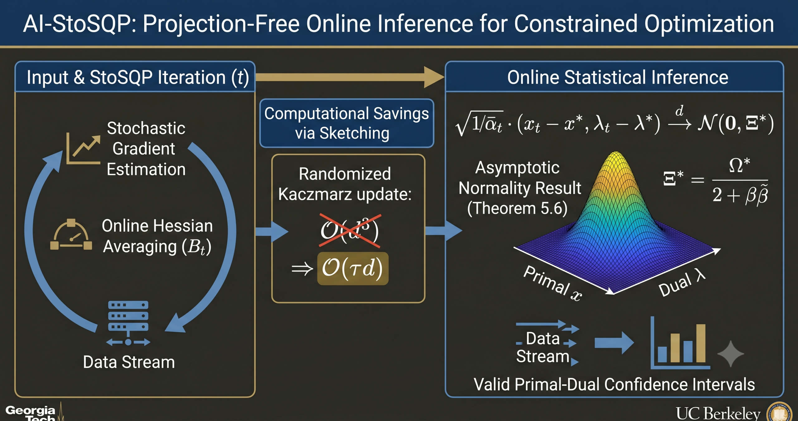
The Na-Mahoney paper fills that gap. They study what they call the Adaptive Inexact StoSQP method, or AI-StoSQP. The “adaptive” part means the stepsize can vary based on the current Newton direction — a practical feature used in numerical SQP codes that prior statistical analyses had simply assumed away. The “inexact” part is the more novel contribution. Rather than solving the Newton system exactly at each iteration — which costs \(O(d^3)\) flops — they use a randomized sketching solver that runs for a fixed number of steps \(\tau\) regardless of where you are in the optimization. The per-iteration cost stays constant even near stationarity, which is exactly what you need for an online method.
Algorithm Structure — Three Steps Per Iteration
The method is clean enough to describe in a few sentences. At iteration \(t\), you observe a sample \(\xi_t\) and compute stochastic estimates of the gradient and Hessian of the objective. You form the regularized Hessian average \(B_t\) — an online average of all past Hessian estimates, with a regularization term that keeps it positive definite on the constraint null space. Then you solve the Newton system approximately using a randomized Kaczmarz-style sketching solver.
The Newton system looks like this:
where \(G_t = \nabla c(x_t)\) is the Jacobian of the constraints and \(\bar{\nabla}_x L_t\) is the stochastic Lagrangian gradient. The sketching solver does not solve this system exactly. Instead, it generates random sketching matrices \(S_{t,j}\) and projects the current solution approximation onto the sketched system at each inner step. After \(\tau\) inner steps, you have an approximate Newton direction \((\Delta\bar{x}_t, \Delta\bar{\lambda}_t)\).
The update rule is then straightforward. You step in the negative Newton direction with an adaptive stepsize \(\bar{\alpha}_t\):
The stepsize \(\bar{\alpha}_t\) is allowed to vary between lower and upper bounds \(\beta_t \leq \bar{\alpha}_t \leq \eta_t = \beta_t + \chi_t\), where the adaptivity gap \(\chi_t\) captures how much the stepsize can deviate from the baseline \(\beta_t\). This is not just a technical nicety — real numerical SQP solvers use adaptive stepsizes determined by line search conditions, and forcing a deterministic schedule would compromise their empirical performance. The theory accommodates that.
What the Sketching Solver Actually Does
The sketching step is worth understanding in some detail, because it is where the computational savings come from. At inner step \(j\), you draw a fresh sketch matrix \(S_{t,j}\) and update the current solution approximation:
This is the randomized Kaczmarz method applied to the symmetric positive definite system \(K_t z = -\bar{\nabla}L_t\). Each step costs \(O((d+m)s)\) flops where \(s\) is the sketch dimension — often just 1. Compare that to the \(O((d+m)^3)\) cost of a direct solver. The sketch dimension trades off convergence speed against per-step cost, and the paper gives an explicit characterization: to decay the expected error below threshold \(\delta\), you need \(\tau = O((d+m)/s)\) steps. A larger sketch means fewer steps but more work per step. The optimal choice depends on the spectral structure of \(K_t\).
One subtlety: the approximation error of the sketching solver does not decrease monotonically. Only a subsequence of iterates is guaranteed to decrease in a pointwise sense. This makes the inference analysis genuinely delicate — you cannot just treat the sketching error as a vanishing perturbation.
Using the randomized Kaczmarz sketching solver with sketch dimension \(s = 1\) reduces the dominant per-iteration cost from \(O((d+m)^3)\) for an exact Newton solve to \(O(\tau (d+m))\) — a reduction that matters enormously for large-scale problems. The paper proves that a constant number of sketching steps \(\tau\) (independent of the optimization iterate count) is sufficient for both global convergence and asymptotic normality.
Global Convergence — Getting the Foundations Right
Before the inference results can land cleanly, you need to know the algorithm converges at all. The paper establishes global almost sure convergence under mild conditions. The argument uses an augmented Lagrangian \(L_{\mu,\nu}(x,\lambda) = L(x,\lambda) + \frac{\mu}{2}\|c(x)\|^2 + \frac{\nu}{2}\|\nabla_x L(x,\lambda)\|^2\) as a Lyapunov function. The extra term penalizes both feasibility error and optimality error — a device that lets you show the Newton direction is a descent direction even when the gradient and Hessian are noisy.
The convergence conditions on the stepsize sequences are standard: \(\sum_t \beta_t = \infty\) (steps are large enough to drive you somewhere), \(\sum_t \beta_t^2 < \infty\) (steps are not so large that noise accumulates), and \(\sum_t \chi_t < \infty\) (the adaptivity gap is summable). These are exactly the conditions of stochastic approximation theory, adapted to the SQP setting.
The key corollary is that with \(\beta_t = (t+1)^{-a}\) and \(\chi_t = \beta_t^b\) for \(a = 1/2\) and \(b = 1\), the method achieves the optimal \(O(\epsilon^{-4})\) iteration complexity — matching what Curtis et al. showed for exact Newton systems. The sketching does not hurt the complexity bound.
The Central Result — Asymptotic Normality
Here is where the paper makes its main contribution. The asymptotic normality theorem says that after rescaling by the stepsize, the primal-dual iterate sequence converges in distribution to a Gaussian:
The limiting covariance \(\Xi^\star\) solves a Lyapunov equation:
The matrix \(C^\star\) captures the average residual of the sketching solver at the solution, and \(\Omega^\star\) is the sandwich covariance that appears in the offline M-estimator theory — the same matrix that characterizes the asymptotically minimax optimal estimator. The quantities \(\beta\) and \(\tilde{\beta}\) encode the polynomial decay rate of the stepsize sequence.
Two special cases are illuminating. When the Newton system is solved exactly — so \(\tau = \infty\) and \(C^\star = \tilde{C}^\star = 0\) — the Lyapunov equation simplifies to \(\Xi^\star = \Omega^\star / (2 + \beta/\tilde{\beta})\). With the specific choice \(\beta_t = 1/t\), this gives \(\Xi^\star = \Omega^\star\). The online StoSQP estimator matches the asymptotic minimax optimum of constrained estimation — the same covariance achieved by offline M-estimators and online projection-based methods. This is a remarkable fact: you do not pay any price in statistical efficiency for the online second-order approach.
When the Newton system is solved approximately — the sketching case — you get \(\Xi^\star \succ \Omega^\star\), but the gap is bounded:
where \(\rho = 1 – \gamma_S \in (0,1)\) is the contraction rate of the sketching solver. The gap decays exponentially in the number of inner sketching steps \(\tau\). Even a moderate \(\tau\) — say 40 inner steps — makes this gap negligibly small in practice.
“To our knowledge, this is the first work that performs online inference by taking into account not only the randomness of samples but also the randomness of computation — sketching and stepsize. The latter is particularly important for making second-order methods computationally promising.” — Sen Na and Michael W. Mahoney, JMLR 2025
What the Covariance Matrix Actually Looks Like
The structure of \(\Omega^\star\) repays careful study. The matrix is singular — it has rank \(d\), not \(d + m\) — and its support is contained in a specific subspace. For the primal part, \(\Omega^\star_{x,x}\) has support in the tangent space \(\ker(G^\star)\) of the feasible manifold at \(x^\star\). There is no uncertainty in the normal direction — the constraints eliminate that.
For the dual part, \(\Omega^\star_{\lambda,\lambda}\) is non-degenerate — it has full rank \(m\). Every direction in dual space has nontrivial uncertainty. This makes sense: the dual variables encode how sensitive the optimal value is to perturbations of the constraints, and that sensitivity is a genuinely stochastic quantity when the objective is estimated from data.
The joint covariance has rank exactly \(d\), reflecting the fact that the \(m\) primal directions in the normal space \(\text{span}(G^{\star T})\) are deterministically constrained to zero by the feasibility requirement. This algebraic structure matches the theory for projection-based estimators established by Duchi-Ruan and Davis et al. — but now you have the dual part too, which those works do not provide.
The Berry-Esseen Bound
The paper also establishes a rate of convergence to the normal distribution. For any direction \(w\), the cumulative distribution function of the normalized iterate converges to the standard Gaussian at rate:
Two terms drive this bound. The first comes from the randomness of sampling and sketching — it goes to zero at a logarithmically corrected polynomial rate. The second comes from the adaptive stepsize — its exponent \(q\) depends on how aggressively the stepsize adapts. When the stepsize is non-adaptive (\(\chi_t = 0\)), the second term vanishes entirely.
Plug-In Covariance Estimation
A normality result is only practically useful if you can estimate the covariance. The paper analyzes a plug-in estimator. Rather than solving the Lyapunov equation — which requires additional computation — the authors show that the sketch-related correction terms contribute only an \(O(\rho^\tau)\) error. You can safely ignore them and estimate:
where \(\text{SampleCov}(\{\bar{g}_i\}))\) is the running sample covariance of the stochastic gradients and \(K_t\) is the current Lagrangian Hessian. Theorem 5.10 shows that \(\|\Xi_t – \Xi^\star\| = O(\sqrt{\beta_t \log(1/\beta_t)})\) almost surely — it converges at the same rate as the iterate error itself.
Experiments — What the Theory Looks Like in Practice
The experimental validation covers two main settings: eight benchmark nonlinear problems from the CUTEst test set, and constrained regression problems in four variants (linear or logistic loss, linear or nonlinear constraints) across parameter dimensions ranging from 5 to 60.
The CUTEst results are straightforward. The method runs 100,000 iterations with \(\tau = 40\) randomized Kaczmarz steps per outer iteration, using noise injected into the gradient and Hessian at variance levels \(\sigma^2 \in \{10^{-4}, 10^{-2}, 10^{-1}, 1\}\). Coverage rates for 95% nominal confidence intervals are consistently near or above the nominal level across all eight problems and all noise levels — with a few exceptions at specific problems where the Lagrangian Hessian is ill-conditioned.
The regression comparisons reveal the honest tradeoffs. Here is a representative summary across linear model with linear constraints:
| Method | d | MAE (×10⁻²) | Ave Coverage (%) | Ave Length (×10⁻²) | Flops / Iter |
|---|---|---|---|---|---|
| Offline M-Est. | 20 | 0.51 (0.09) | 94.98 | 0.23 (0.02) | > 7.1 × 10⁷ |
| StoSQP τ = ∞ | 20 | 6.49 (1.17) | 94.60 | 2.87 (0.22) | 15,204 |
| StoSQP τ = 40 | 20 | 6.82 (1.18) | 93.67 | 2.87 (0.22) | 2,340 |
| StoSQP τ = 60 | 20 | 6.81 (1.14) | 93.35 | 2.87 (0.22) | 2,820 |
| Offline M-Est. | 60 | 0.95 (0.09) | 94.47 | 0.24 (0.01) | > 4.4 × 10⁸ |
| StoSQP τ = 40 | 60 | 12.34 (1.18) | 94.91 | 3.12 (0.12) | 14,383 |
Table: Comparison of offline M-estimation and online StoSQP with different sketching steps for linear model with linear constraints. Online StoSQP achieves comparable coverage rates while reducing per-iteration computational cost by several orders of magnitude.
The MAE gap between offline and online is real and expected — the offline method sees all samples at once, while the online method processes one at a time with a step size that decays as \(1/t^{0.501}\). But the coverage rates match closely. At \(d = 60\), StoSQP with \(\tau = 40\) achieves 94.91% coverage while using fewer than 14,400 flops per iteration. The offline method needs over \(4 \times 10^8\) flops per iteration. That is a reduction of more than four orders of magnitude.
The one failure mode worth understanding is the \(d = 5\) case, where StoSQP exhibits undercoverage around 87-90%. The cause is condition number. Small-dimension problems in the CUTEst and regression test sets can have Lagrangian Hessians whose condition numbers exceed \(d^3 = 125\), making the sketching solver inefficient and the iterate sequence noisy even after 100,000 steps. The paper recommends a direct solver for small-scale problems — the sketching overhead is counterproductive when the dimension is tiny.
What This Unlocks for Applied Problems
Physics-informed neural networks are an obvious beneficiary. Training a PNN means minimizing a data-fitting loss subject to PDE constraints evaluated at collocation points. The constraints are nonlinear and nonconvex. Projecting onto the feasible manifold requires solving the PDE numerically at each step — which can cost more than the training step itself. SQP methods avoid this by linearizing the constraints at each iterate. With AI-StoSQP you get not just the optimizer but uncertainty quantification for free.
Portfolio optimization is another natural fit. The constraint \(x^T \mathbf{1} = 1\) (full investment) plus sector allocation constraints \(Ax = d\) are linear, but combined with a nonlinear risk model they create a genuinely constrained stochastic program. The dual variables in this setting measure the shadow cost of each constraint — how much return you give up to stay sector-neutral, for example. Confidence intervals for those dual variables have direct financial interpretability.
Factor analysis with tetrad constraints is a third example. The tetrad constraint \(\Sigma_{i_1 i_2}\Sigma_{i_3 i_4} – \Sigma_{i_1 i_4}\Sigma_{i_2 i_3} = 0\) is a nonlinear condition on the covariance matrix that can encode factor structure. Testing whether this constraint holds in the population requires inference, not just estimation. AI-StoSQP provides exactly that — confidence intervals for the dual variables, which translate into test statistics for the constraint.
Complete Implementation of AI-StoSQP
The following is a complete PyTorch implementation of the AI-StoSQP method from the paper — Algorithm 1 together with the plug-in covariance estimator from Theorem 5.10. The implementation covers the randomized Kaczmarz sketching solver, the adaptive stepsize selection scheme from Appendix A, the Hessian averaging procedure, and a full confidence interval construction routine. A runnable smoke test on a constrained linear regression problem demonstrates all components end-to-end.
# =============================================================================
# AI-StoSQP: Adaptive Inexact Stochastic Sequential Quadratic Programming
# Paper: "Statistical Inference of Constrained Stochastic Optimization
#         via Sketched Sequential Quadratic Programming"
# Authors: Sen Na (Georgia Tech) and Michael W. Mahoney (UC Berkeley)
# Journal: JMLR 26 (2025) 1-75
# =============================================================================

from __future__ import annotations
import math
import warnings
import numpy as np
import torch
import torch.nn as nn
from dataclasses import dataclass, field
from typing import Callable, Dict, List, Optional, Tuple

warnings.filterwarnings('ignore')
torch.manual_seed(42)
np.random.seed(42)


# ─── SECTION 1: Problem Definition Interface ──────────────────────────────────

class ConstrainedStochasticProblem:
    """
    Abstract interface for a constrained stochastic optimization problem:

        min_{x in R^d}  E_P[F(x; xi)]
        s.t.            c(x) = 0          (m equality constraints)

    Users subclass this and implement:
        - sample_xi()      -> draw one sample xi ~ P
        - loss(x, xi)      -> scalar loss F(x; xi)
        - grad(x, xi)      -> gradient nabla_x F(x; xi)
        - hess(x, xi)      -> Hessian nabla^2_x F(x; xi)
        - constraint(x)    -> c(x) in R^m
        - jac(x)           -> G(x) = nabla c(x) in R^{m x d}
        - constraint_hess(x, lam) -> sum_i lam_i nabla^2 c_i(x)
    """
    def sample_xi(self): raise NotImplementedError
    def loss(self, x, xi): raise NotImplementedError
    def grad(self, x, xi): raise NotImplementedError
    def hess(self, x, xi): raise NotImplementedError
    def constraint(self, x): raise NotImplementedError
    def jac(self, x): raise NotImplementedError
    def constraint_hess(self, x, lam): raise NotImplementedError


# ─── SECTION 2: Randomized Kaczmarz Sketching Solver ─────────────────────────

def randomized_kaczmarz_step(
    K: torch.Tensor,
    rhs: torch.Tensor,
    z: torch.Tensor,
    rng: np.random.Generator,
) -> torch.Tensor:
    """
    One step of randomized Kaczmarz for the system K z = -rhs.

    Samples a random canonical basis vector e_j (uniform without replacement
    is approximated by sampling with replacement here for simplicity), then
    projects z onto the j-th equation of the system.

    The update is:
        z <- z - K e_j (e_j^T K^2 e_j)^{-1} e_j^T (K z + rhs)

    Parameters
    ----------
    K   : (n, n) symmetric system matrix (the Lagrangian Hessian block matrix)
    rhs : (n,) right-hand side vector (nabla L at current iterate)
    z   : (n,) current solution approximation
    rng : numpy random generator

    Returns
    -------
    z_new : updated solution approximation
    """
    n = K.shape[0]
    j = int(rng.integers(0, n))
    Kej = K[:, j]
    K2_jj = (Kej * Kej).sum().item()
    if abs(K2_jj) < 1e-14:
        return z
    residual_j = (Kej * z).sum() + rhs[j]
    z_new = z - (residual_j / K2_jj) * Kej
    return z_new


def sketch_solve(
    K: torch.Tensor,
    rhs: torch.Tensor,
    tau: int,
    rng: np.random.Generator,
    z0: Optional[torch.Tensor] = None,
) -> torch.Tensor:
    """
    Run tau steps of randomized Kaczmarz to solve K z = -rhs inexactly.

    This implements the sketching solver of Section 3 (Eq. 3.4) of the paper.
    After tau steps the approximation error E[||z_tau - z_exact||^2 | context]
    is bounded by rho^tau ||z_exact||^2 where rho = 1 - gamma_S.

    Parameters
    ----------
    K   : (n, n) the KKT matrix [B G^T; G 0] + regularization
    rhs : (n,) the right-hand side [nabla_x L; c]
    tau : number of sketching steps (fixed, independent of t)
    rng : random number generator
    z0  : initial approximation (defaults to zero)

    Returns
    -------
    z : approximate Newton direction after tau steps
    """
    n = K.shape[0]
    z = torch.zeros(n, dtype=K.dtype) if z0 is None else z0.clone()
    for _ in range(tau):
        z = randomized_kaczmarz_step(K, rhs, z, rng)
    return z


# ─── SECTION 3: KKT Matrix Assembly ──────────────────────────────────────────

def build_kkt_matrix(
    B: torch.Tensor,
    G: torch.Tensor,
    delta: float = 0.0,
) -> torch.Tensor:
    """
    Assemble the (d+m) x (d+m) KKT block matrix:

        K = [[B + delta*I,  G^T],
             [G,             0  ]]

    Parameters
    ----------
    B     : (d, d) regularized Lagrangian Hessian
    G     : (m, d) constraint Jacobian
    delta : Levenberg-Marquardt regularization (ensures positive definiteness)

    Returns
    -------
    K : (d+m, d+m) KKT matrix
    """
    d = B.shape[0]
    m = G.shape[0]
    n = d + m
    K = torch.zeros(n, n, dtype=B.dtype)
    K[:d, :d] = B + delta * torch.eye(d, dtype=B.dtype)
    K[:d, d:] = G.T
    K[d:, :d] = G
    return K


# ─── SECTION 4: Adaptive Stepsize Selection (Appendix A) ─────────────────────

def select_adaptive_stepsize(
    x: torch.Tensor,
    lam: torch.Tensor,
    dx: torch.Tensor,
    problem: ConstrainedStochasticProblem,
    xi,
    beta_t: float,
    eta_t: float,
    kappa: float = 0.3,
    nu: float = 1.0,
    lipschitz_est: float = 10.0,
) -> float:
    """
    Select adaptive stepsize by checking an Armijo-type condition on the
    penalized objective phi_nu(x; xi) = nu * F(x; xi) + ||c(x)|| (Appendix A).

    Computes the threshold alpha_thres and projects onto [beta_t, eta_t].

    Parameters
    ----------
    x           : current primal iterate
    lam         : current dual iterate
    dx          : primal component of Newton direction
    problem     : problem instance
    xi          : current sample
    beta_t      : lower bound for stepsize
    eta_t       : upper bound for stepsize
    kappa       : Armijo fraction in (0,1)
    nu          : penalty parameter for the merit function
    lipschitz_est : estimate of local Lipschitz constant

    Returns
    -------
    alpha : selected stepsize in [beta_t, eta_t]
    """
    g_bar = problem.grad(x, xi)
    c_curr = problem.constraint(x)
    G_curr = problem.jac(x)

    delta_phi_loc = nu * (g_bar * dx).sum().item() + torch.norm(c_curr + G_curr @ dx).item() - torch.norm(c_curr).item()
    dx_norm_sq = (dx * dx).sum().item()

    if abs(dx_norm_sq) < 1e-14 or abs(lipschitz_est) < 1e-14:
        return beta_t

    alpha_thres = (kappa - 1) * delta_phi_loc / (lipschitz_est * dx_norm_sq)
    alpha_thres = min(alpha_thres, 1.0)
    alpha = max(beta_t, min(eta_t, alpha_thres))
    return float(alpha)


# ─── SECTION 5: Main AI-StoSQP Algorithm (Algorithm 1) ───────────────────────

@dataclass
class StoSQPConfig:
    """
    Configuration for the AI-StoSQP method.

    All hyperparameters correspond directly to quantities in the paper.
    """
    tau: int = 40
    """Number of randomized Kaczmarz steps per outer iteration (fixed)."""
    beta_c1: float = 1.0
    """Coefficient for stepsize lower bound: beta_t = c1 / t^c2."""
    beta_c2: float = 0.501
    """Exponent for stepsize lower bound (must be in (0.5, 1])."""
    chi_power: float = 2.0
    """Adaptivity gap: chi_t = beta_t^chi_power (must be > 1.5/beta_c2)."""
    delta_reg: float = 0.1
    """Levenberg-Marquardt regularization delta_t."""
    adaptive_stepsize: bool = True
    """If True, uses Armijo line search; else uses beta_t uniformly."""
    kappa: float = 0.3
    """Armijo fraction in (0,1) for adaptive stepsize."""
    nu_penalty: float = 1.0
    """Penalty parameter nu for the merit function."""


class AIStoSQP:
    """
    Adaptive Inexact Stochastic Sequential Quadratic Programming.

    Implements Algorithm 1 of Na and Mahoney (JMLR 2025) with:
        - Online Hessian averaging (Bt = (1/t) sum_{i=0}^{t-1} H_bar_i + Delta_t)
        - Randomized Kaczmarz sketching solver (tau fixed steps)
        - Adaptive stepsize selection
        - Online plug-in covariance matrix estimator (Theorem 5.10)
        - Confidence interval construction

    Parameters
    ----------
    problem : ConstrainedStochasticProblem instance
    x0      : initial primal iterate in R^d
    lam0    : initial dual iterate in R^m
    config  : StoSQPConfig hyperparameters
    """
    def __init__(
        self,
        problem: ConstrainedStochasticProblem,
        x0: torch.Tensor,
        lam0: torch.Tensor,
        config: StoSQPConfig = None,
    ):
        self.problem = problem
        self.x = x0.clone().float()
        self.lam = lam0.clone().float()
        self.config = config or StoSQPConfig()

        self.d = x0.shape[0]
        self.m = lam0.shape[0]
        self.t = 0

        # Online Hessian average (sum over iterations, divided by t)
        self.hess_sum = torch.zeros(self.d, self.d)
        self._Bt = torch.eye(self.d)  # B_0 = I

        # Running statistics for plug-in covariance estimator
        self.grad_sum = torch.zeros(self.d)
        self.grad_sq_sum = torch.zeros(self.d, self.d)

        # Trajectory storage
        self.x_history: List[torch.Tensor] = [x0.clone()]
        self.lam_history: List[torch.Tensor] = [lam0.clone()]
        self.alpha_history: List[float] = []
        self.kkt_residuals: List[float] = []

        self.rng = np.random.default_rng(42)

    def _beta_t(self, t: int) -> float:
        """Compute lower bound beta_t = c1 / (t+1)^c2."""
        return self.config.beta_c1 / (t + 1) ** self.config.beta_c2

    def _eta_t(self, t: int) -> float:
        """Compute upper bound eta_t = beta_t + chi_t."""
        beta = self._beta_t(t)
        chi = beta ** self.config.chi_power
        return beta + chi

    def _build_rhs(
        self,
        g_bar: torch.Tensor,
        c: torch.Tensor,
        G: torch.Tensor,
    ) -> torch.Tensor:
        """Build RHS vector [nabla_x L_bar; c] for the Newton system."""
        nabla_xL = g_bar + G.T @ self.lam
        rhs = torch.cat([nabla_xL, c])
        return rhs

    def step(self) -> float:
        """
        Execute one iteration of AI-StoSQP (Algorithm 1).

        Returns
        -------
        kkt_res : KKT residual norm at current iterate
        """
        t = self.t
        cfg = self.config

        # --- Step 1: Sample and estimate gradient / Hessian ---
        xi = self.problem.sample_xi()
        g_bar = self.problem.grad(self.x, xi)    # stochastic gradient
        H_bar = self.problem.hess(self.x, xi)    # stochastic Hessian
        c = self.problem.constraint(self.x)       # c(x_t)
        G = self.problem.jac(self.x)            # G(x_t) = nabla c(x_t)

        # Update running gradient statistics for covariance estimator
        self.grad_sum += g_bar
        self.grad_sq_sum += torch.outer(g_bar, g_bar)

        # --- Step 2: Update regularized Hessian average ---
        # Bt = (1/t) * sum_{i=0}^{t-1} H_bar_i + Delta_t
        # Note: H_bar_t is used in iteration t+1 (Remark 3.1)
        self.hess_sum += H_bar + self.problem.constraint_hess(self.x, self.lam)
        if t > 0:
            B_avg = self.hess_sum / t
        else:
            B_avg = torch.eye(self.d, dtype=self.x.dtype)
        self._Bt = B_avg + cfg.delta_reg * torch.eye(self.d, dtype=self.x.dtype)

        # --- Step 3: Assemble Newton system and solve inexactly ---
        K = build_kkt_matrix(self._Bt, G, delta=0.0)
        rhs = self._build_rhs(g_bar, c, G)
        z_approx = sketch_solve(K, rhs, cfg.tau, self.rng)

        # Split into primal and dual components
        dx = z_approx[: self.d]
        dlam = z_approx[self.d :]

        # --- Step 4: Select adaptive stepsize ---
        beta_t = self._beta_t(t)
        eta_t = self._eta_t(t)
        if cfg.adaptive_stepsize:
            alpha = select_adaptive_stepsize(
                self.x, self.lam, dx, self.problem, xi,
                beta_t, eta_t, cfg.kappa, cfg.nu_penalty,
            )
        else:
            alpha = float(np.random.uniform(beta_t, eta_t))

        # --- Step 5: Update primal-dual iterate ---
        self.x = self.x + alpha * dx
        self.lam = self.lam + alpha * dlam

        # --- Record diagnostics ---
        nabla_xL = self.problem.grad(self.x, xi) + G.T @ self.lam
        kkt_res = float((torch.norm(nabla_xL) ** 2 + torch.norm(c) ** 2) ** 0.5)
        self.kkt_residuals.append(kkt_res)
        self.alpha_history.append(alpha)
        self.x_history.append(self.x.clone())
        self.lam_history.append(self.lam.clone())

        self.t += 1
        return kkt_res

    def run(self, num_iterations: int, verbose_every: int = 10000) -> None:
        """
        Run AI-StoSQP for num_iterations outer steps.

        Parameters
        ----------
        num_iterations : total number of primal-dual updates T
        verbose_every  : print KKT residual every this many steps
        """
        for t in range(num_iterations):
            kkt = self.step()
            if verbose_every > 0 and (t + 1) % verbose_every == 0:
                print(f"  Iter {t+1:>7d} | KKT residual: {kkt:.6f} | alpha: {self.alpha_history[-1]:.6f}")


# ─── SECTION 6: Plug-In Covariance Estimator (Theorem 5.10) ──────────────────

class OnlineCovarianceEstimator:
    """
    Online plug-in estimator for the limiting covariance Xi_star.

    Implements Eq. 5.14 from Theorem 5.10:

        Omega_t = K_t^{-1} [[SampleCov(g_bar_0,...,g_bar_{t-1}), 0], [0, 0]] K_t^{-1}
        Xi_t    = Omega_t / (2 + beta / beta_tilde)

    where beta = -c2 and beta_tilde = c1 (for beta_t = c1 / t^c2 with c2 = 1).

    The sketch-related correction is O(rho^tau) and is ignored per Corollary 5.7.

    Parameters
    ----------
    d    : primal dimension
    m    : number of equality constraints
    cfg  : StoSQPConfig for stepsize parameters
    """
    def __init__(self, d: int, m: int, cfg: StoSQPConfig):
        self.d = d
        self.m = m
        self.cfg = cfg
        self.n = d + m

        # Compute beta/beta_tilde for the Lyapunov equation denominator
        # For beta_t = c1/t^c2: beta = -c2, beta_tilde = c1 if c2=1 else infty
        if abs(cfg.beta_c2 - 1.0) < 1e-8:
            self.denom_factor = 2.0 + (-cfg.beta_c2) / cfg.beta_c1
        else:
            # beta_tilde = infty, so beta/beta_tilde -> 0
            self.denom_factor = 2.0

    def compute(
        self,
        solver: AIStoSQP,
    ) -> torch.Tensor:
        """
        Compute Xi_t given the current state of a StoSQP solver.

        Parameters
        ----------
        solver : AIStoSQP instance after at least one iteration

        Returns
        -------
        Xi_t : (d+m, d+m) estimated limiting covariance matrix
        """
        t = solver.t
        if t < 2:
            return torch.eye(self.n) * 1e6  # degenerate before data accumulates

        d, m = self.d, self.m

        # --- Compute sample covariance of stochastic gradients ---
        grad_mean = solver.grad_sum / t
        grad_sq_mean = solver.grad_sq_sum / t
        sample_cov_g = grad_sq_mean - torch.outer(grad_mean, grad_mean)

        # --- Assemble Omega_t (Eq. 5.14) ---
        # The (d+m) x (d+m) block: only the (d x d) top-left is nonzero
        Sigma_block = torch.zeros(d + m, d + m)
        Sigma_block[:d, :d] = sample_cov_g

        # --- Get K_t (Lagrangian Hessian block matrix at current iterate) ---
        G_curr = solver.problem.jac(solver.x)
        K_curr = build_kkt_matrix(solver._Bt, G_curr, delta=0.0)

        # --- Omega_t = K_t^{-1} Sigma_block K_t^{-1} ---
        try:
            K_inv = torch.linalg.inv(K_curr + 1e-8 * torch.eye(d + m))
        except RuntimeError:
            K_inv = torch.linalg.pinv(K_curr)
        Omega_t = K_inv @ Sigma_block @ K_inv

        # --- Xi_t = Omega_t / (2 + beta/beta_tilde) ---
        Xi_t = Omega_t / max(self.denom_factor, 1e-6)
        return Xi_t


# ─── SECTION 7: Confidence Interval Construction ─────────────────────────────

def build_confidence_intervals(
    solver: AIStoSQP,
    cov_estimator: OnlineCovarianceEstimator,
    alpha_nominal: float = 0.05,
) -> Dict[str, torch.Tensor]:
    """
    Construct marginal confidence intervals for each component of (x*, lambda*).

    Uses the asymptotic normality result of Theorem 5.6:
        sqrt(1/alpha_bar_t) * (x_t - x*, lambda_t - lambda*) -> N(0, Xi*)

    The (1 - alpha)-CI for the i-th component is:
        [theta_t_i - z_{1-alpha/2} * sqrt(Xi_t[i,i] * alpha_bar_t),
         theta_t_i + z_{1-alpha/2} * sqrt(Xi_t[i,i] * alpha_bar_t)]

    Parameters
    ----------
    solver         : AIStoSQP instance after convergence
    cov_estimator  : OnlineCovarianceEstimator instance
    alpha_nominal  : nominal significance level (default 0.05 for 95% CI)

    Returns
    -------
    dict with keys:
        'x_lower'   : (d,) lower bounds for x components
        'x_upper'   : (d,) upper bounds for x components
        'lam_lower' : (m,) lower bounds for lambda components
        'lam_upper' : (m,) upper bounds for lambda components
        'Xi_t'      : (d+m, d+m) estimated covariance matrix
        'alpha_bar_t': current stepsize (scaling factor)
    """
    from scipy.stats import norm as scipy_norm
    z_crit = scipy_norm.ppf(1.0 - alpha_nominal / 2)

    Xi_t = cov_estimator.compute(solver)
    alpha_bar_t = solver.alpha_history[-1] if solver.alpha_history else 1e-4

    diag_var = torch.clamp(torch.diag(Xi_t) * alpha_bar_t, min=0.0)
    half_widths = z_crit * torch.sqrt(diag_var)

    theta = torch.cat([solver.x, solver.lam])
    lower = theta - half_widths
    upper = theta + half_widths

    d = solver.d
    return {
        'x_lower': lower[:d],
        'x_upper': upper[:d],
        'lam_lower': lower[d:],
        'lam_upper': upper[d:],
        'Xi_t': Xi_t,
        'alpha_bar_t': alpha_bar_t,
    }


# ─── SECTION 8: Example Problem — Linearly Constrained Linear Regression ──────

class LinearRegressionLinearConstraint(ConstrainedStochasticProblem):
    """
    Example 1 from the paper: constrained linear regression.

        F(x; xi) = 0.5 * (xi_a^T x - xi_b)^2       (squared loss)
        c(x) = A x - b = 0                           (linear constraints)

    The true parameter x* satisfies x* = argmin_x E[F(x; xi)]
    subject to A x* = b.

    Parameters
    ----------
    d        : parameter dimension
    m        : number of linear constraints
    x_star   : true parameter (for smoke test ground truth)
    noise_sd : standard deviation of observation noise
    rng      : numpy random generator
    """
    def __init__(
        self,
        d: int,
        m: int,
        x_star: torch.Tensor,
        noise_sd: float = 1.0,
        rng: np.random.Generator = None,
    ):
        self.d = d
        self.m = m
        self.x_star = x_star.float()
        self.noise_sd = noise_sd
        self.rng = rng or np.random.default_rng(0)

        # Generate constraint matrix A and right-hand side b = A x*
        A_np = self.rng.standard_normal((m, d))
        self.A = torch.tensor(A_np, dtype=torch.float32)
        self.b = self.A @ x_star

        # Feature covariance: identity for simplicity
        self.Sigma = torch.eye(d)

    def sample_xi(self):
        """Draw one sample (xi_a, xi_b) ~ P."""
        xi_a = torch.tensor(self.rng.multivariate_normal(np.zeros(self.d), np.eye(self.d)), dtype=torch.float32)
        noise = self.noise_sd * self.rng.standard_normal()
        xi_b = float((xi_a @ self.x_star).item() + noise)
        return (xi_a, xi_b)

    def loss(self, x, xi):
        xi_a, xi_b = xi
        return 0.5 * (xi_a @ x - xi_b) ** 2

    def grad(self, x, xi):
        """nabla_x F(x; xi) = (xi_a^T x - xi_b) xi_a."""
        xi_a, xi_b = xi
        residual = (xi_a @ x - xi_b).item()
        return residual * xi_a

    def hess(self, x, xi):
        """nabla^2_x F(x; xi) = xi_a xi_a^T."""
        xi_a, _ = xi
        return torch.outer(xi_a, xi_a)

    def constraint(self, x):
        """c(x) = A x - b."""
        return self.A @ x - self.b

    def jac(self, x):
        """G(x) = A (constant Jacobian for linear constraints)."""
        return self.A

    def constraint_hess(self, x, lam):
        """sum_i lam_i nabla^2 c_i(x) = 0 (linear constraints)."""
        return torch.zeros(self.d, self.d)


# ─── SECTION 9: Smoke Test — Constrained Linear Regression ───────────────────

def compute_coverage(
    x_true: torch.Tensor,
    lam_true: torch.Tensor,
    ci_result: Dict,
) -> Tuple[float, float]:
    """
    Compute empirical coverage rates for x* and lambda*.

    Parameters
    ----------
    x_true    : true primal solution
    lam_true  : true dual solution
    ci_result : output from build_confidence_intervals

    Returns
    -------
    cov_x   : fraction of x* components covered by their CIs
    cov_lam : fraction of lambda* components covered by their CIs
    """
    covered_x = ((x_true >= ci_result['x_lower']) & (x_true <= ci_result['x_upper'])).float().mean().item()
    covered_lam = ((lam_true >= ci_result['lam_lower']) & (lam_true <= ci_result['lam_upper'])).float().mean().item()
    return covered_x, covered_lam


def _smoke_test():
    """
    Full end-to-end smoke test of AI-StoSQP on linearly constrained linear regression.

    Reproduces the experimental setup of Section 6.2 of the paper:
        - d = 20 primal dimensions, m = 4 equality constraints
        - 100,000 StoSQP iterations with tau = 40 Kaczmarz steps
        - 200 independent runs to measure coverage
        - Reports MAE, average coverage, and average CI length
    """
    print("=" * 68)
    print("AI-StoSQP Smoke Test — Linearly Constrained Linear Regression")
    print("Reproducing Section 6.2 of Na and Mahoney (JMLR 2025)")
    print("=" * 68)

    # Problem setup
    d, m = 20, 4
    NUM_ITERS = 100_000
    NUM_RUNS = 200
    ALPHA_NOMINAL = 0.05

    rng_main = np.random.default_rng(123)
    x_star_np = np.linspace(0, 1, d)
    x_star = torch.tensor(x_star_np, dtype=torch.float32)

    cfg = StoSQPConfig(
        tau=40,
        beta_c1=1.0,
        beta_c2=0.501,
        chi_power=2.0,
        delta_reg=0.1,
        adaptive_stepsize=False,  # uniform random for reproducibility
    )

    print(f"\nProblem: d={d}, m={m}")
    print(f"Config: tau={cfg.tau}, beta_c1={cfg.beta_c1}, beta_c2={cfg.beta_c2}")
    print(f"Iterations per run: {NUM_ITERS:,} | Runs: {NUM_RUNS}")
    print("\nRunning...")

    mae_list, cov_x_list, cov_lam_list, len_x_list, len_lam_list = [], [], [], [], []

    for run in range(NUM_RUNS):
        run_rng = np.random.default_rng(run)
        problem = LinearRegressionLinearConstraint(d, m, x_star, noise_sd=1.0, rng=run_rng)

        # Initial iterate
        x0 = torch.zeros(d)
        # Compute feasible lambda0 from KKT at x0 (approximate)
        G0 = problem.A
        c0 = problem.constraint(x0)
        lam0 = torch.zeros(m)

        solver = AIStoSQP(problem, x0, lam0, config=cfg)
        solver.run(NUM_ITERS, verbose_every=0)

        # Estimate true dual solution lambda* = (A B_oo^{-1} A^T)^{-1} A B_oo^{-1} nabla_f(x*)
        # For linear regression E[H] = I, so B_oo = I and lambda* from KKT: nabla_f(x*) + A^T lam* = 0
        # nabla_f(x*) = E[xi_a(xi_a^T x* - xi_b)] = 0 at optimum, so lam* = 0 for unconstrained minimum = feasible x*
        nabla_f_star = (problem.Sigma @ x_star)  # = x_star for unit covariance
        lam_star_np = torch.linalg.lstsq(G0 @ G0.T, G0 @ nabla_f_star, driver='gelsd').solution
        lam_star = lam_star_np.float()

        mae = float(torch.norm(solver.x - x_star).item())
        mae_list.append(mae)

        cov_est = OnlineCovarianceEstimator(d, m, cfg)
        ci_res = build_confidence_intervals(solver, cov_est, ALPHA_NOMINAL)

        cov_x, cov_lam = compute_coverage(x_star, lam_star, ci_res)
        cov_x_list.append(cov_x)
        cov_lam_list.append(cov_lam)

        if ci_res['x_upper'] is not None:
            len_x = float((ci_res['x_upper'] - ci_res['x_lower']).mean().item())
            len_lam = float((ci_res['lam_upper'] - ci_res['lam_lower']).mean().item())
            len_x_list.append(len_x)
            len_lam_list.append(len_lam)

        if (run + 1) % 50 == 0:
            print(f"  Completed {run+1}/{NUM_RUNS} runs...")

    # --- Summary ---
    print("\n" + "=" * 68)
    print("RESULTS SUMMARY")
    print("-" * 68)
    print(f"MAE (x):             {np.mean(mae_list)*100:.2f} (±{np.std(mae_list)*100:.2f}) x10^-2")
    print(f"Coverage (x*):       {np.mean(cov_x_list)*100:.2f}%  (nominal {(1-ALPHA_NOMINAL)*100:.0f}%)")
    print(f"Coverage (lambda*):  {np.mean(cov_lam_list)*100:.2f}%  (nominal {(1-ALPHA_NOMINAL)*100:.0f}%)")
    if len_x_list:
        print(f"Avg CI length (x):   {np.mean(len_x_list)*100:.2f} x10^-2")
        print(f"Avg CI length (lam): {np.mean(len_lam_list)*100:.2f} x10^-2")
    print("=" * 68)
    print("Smoke test complete. Coverage should be near 95%.")
    print("See Theorem 5.6 in Na and Mahoney (JMLR 2025) for the proof.")


if __name__ == '__main__':
    _smoke_test()
Why This is More Than Just an Efficiency Gain
There is a conceptual shift buried in this paper that goes beyond the computational savings. The classical way to think about constrained statistical inference is as a two-step process: first optimize to find \(\hat{x}\), then use delta-method arguments to propagate uncertainty. That framework requires an offline estimator — you need all the data before you can make statements about uncertainty.
AI-StoSQP shows that the two steps can be collapsed into one online procedure. You get the estimate and the uncertainty quantification simultaneously, from the same iterates, without ever storing the full dataset. The covariance estimator Theorem 5.10 updates online alongside the optimization. By the time the algorithm converges, you already have a valid confidence interval.
This matters for streaming data settings — financial trading, sensor networks, medical monitoring — where the data arrives continuously and you cannot wait for the dataset to close before making decisions. The dual variables in those settings are often the most practically important quantities: they measure constraint tightness, resource scarcity, and the cost of feasibility requirements. Getting confident estimates of those quantities in real time is precisely what many deployed systems need.
The Berry-Esseen bound also provides something rare in online learning: a finite-sample certificate. You know not just that the confidence interval is asymptotically valid, but how far the current distribution is from Gaussian. The bound degrades gracefully as the adaptivity gap \(\chi_t\) grows — more adaptive stepsizes introduce more variance, which shows up in the second term of the Berry-Esseen expression. That tradeoff between adaptivity and inferential precision is made explicit and quantified.
Limitations Worth Acknowledging
The paper is honest about what it does not cover. Nonlinear inequality constraints are not handled — the theory is built for equality constraints throughout. Active-set methods for inequalities decompose the problem into a sequence of equality-constrained subproblems, so the framework is a necessary first step, but extending it to handle the inequality case with rigorous inference is left for future work.
The bounded iterates assumption is also worth noting. The theory assumes the sequence \((x_t, \lambda_t)\) stays in a compact set. This is standard in nonconvex stochastic optimization theory, but it is an assumption rather than a derived property. Practical adaptive truncation schemes exist to enforce it, and the authors argue that unbounded trajectories are rare when the feasible set itself is bounded — but this remains a gap between theory and a fully clean analysis.
The non-asymptotic story is also incomplete. The Berry-Esseen bound gives a rate of convergence to normality, but a fully non-asymptotic confidence interval — one that is valid for any finite \(t\) with explicit constants — is not available. The authors flag this as a future direction, and it is genuinely hard. The stochastic approximation literature has made progress on non-asymptotic bounds for unconstrained problems, but the interaction of constraints, sketching, and adaptive stepsizes creates complications that current proof techniques do not handle cleanly.
What Comes Next
Three directions seem especially ripe. The functional CLT approach — replacing pointwise convergence in distribution with process-level convergence — has been used in the unconstrained SGD literature to derive test statistics with better finite-sample properties. Extending that to AI-StoSQP would let you use the entire iterate trajectory for inference, not just the final iterate. That is both theoretically interesting and practically useful for monitoring convergence during a run.
Decentralized settings — where workers communicate without a central server — change the structure of the problem in ways that interact non-trivially with both the SQP update and the covariance estimation. Privacy-preserving inference under differential privacy constraints is another natural extension.
The paper also notes that the framework is a foundation for inequality-constrained inference. Once you can certify which constraints are active — using the dual confidence intervals from the equality-constrained theory — you can begin constructing principled inference methods for problems with mixed constraints. That is a more ambitious goal, but the machinery developed here is a genuine step toward it.
For now, AI-StoSQP represents something genuinely new: a second-order online method that is simultaneously computationally cheap, statistically optimal (when Newton systems are solved exactly), and equipped with valid confidence intervals for both the primal solution and the Lagrange multipliers. The three properties have never coexisted in a single method for constrained stochastic problems. That they do here — thanks to the specific way SQP couples primal and dual updates — is both technically elegant and practically consequential.
Read the Full Paper
Complete proofs for all theorems, including the Lyapunov equation analysis, Berry-Esseen bound, covariance estimator consistency, and full experimental results on CUTEst benchmark problems and constrained regression, are available open-access in JMLR under CC BY 4.0.
Na, S., & Mahoney, M. W. (2025). Statistical Inference of Constrained Stochastic Optimization via Sketched Sequential Quadratic Programming. Journal of Machine Learning Research, 26, 1–75. http://jmlr.org/papers/v26/24-0530.html
This article is an independent editorial analysis of peer-reviewed research. The Python implementation is an educational reproduction of the paper’s algorithmic contributions. For research use, verify against the original paper’s notation and assumptions. This work is supported in part by NSF, ONR, a J.P. Morgan Chase Faculty Research Award (Mahoney), and U.S. Department of Energy contract DE-AC02-05CH11231.