The ODE Method Gets Its Markovian Upgrade — and Reinforcement Learning’s Most Stubborn Problem Finally Has a Clean Answer
A team from the University of Virginia and Scaled Foundations has extended the celebrated Borkar-Meyn theorem to handle Markovian noise, unlocking the first rigorous almost-sure convergence guarantees for GTD(λ) and ETD(λ) — the two principal algorithms for tackling the deadly triad in off-policy RL.
For roughly thirty years, reinforcement learning researchers faced an uncomfortable gap between what their algorithms could do and what they could prove. Off-policy temporal difference methods with eligibility traces work beautifully in practice, but their convergence theory kept running into a wall: the standard mathematical tools for stochastic approximation were all built for independent or Martingale difference noise, and the noise in these algorithms is emphatically neither. Shuze Daniel Liu, Shuhang Chen, and Shangtong Zhang have now closed that gap. Their paper, published in JMLR in 2025, extends the Borkar-Meyn stability theorem to the Markovian noise setting under assumptions that actually hold for the algorithms researchers care about — and the payoff is immediate: the first clean, bias-free almost-sure convergence proofs for GTD(λ) and ETD(λ).
Why This Problem Existed at All
Stochastic approximation is the umbrella framework that covers a huge swath of machine learning — stochastic gradient descent, Q-learning, temporal difference methods, and much more. The basic update rule is deceptively simple:
You have a vector \(x_n\), a sequence of random “noise” inputs \(\{Y_n\}\), a function \(H\) that maps your current state and the noise to an increment, and a shrinking learning rate \(\alpha(n)\). The deep question is: does this sequence converge, and to what?
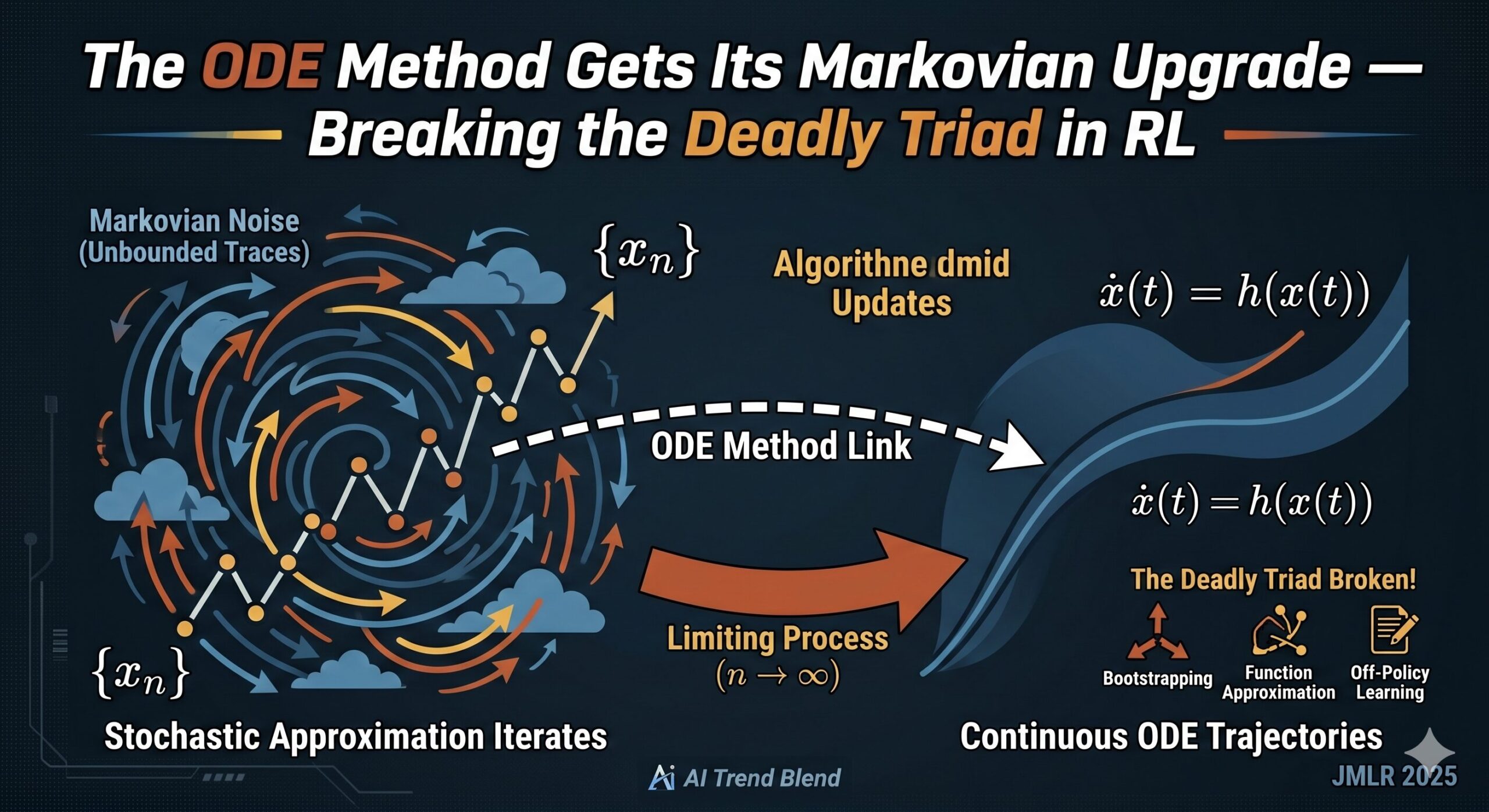
The answer, broadly, comes from the ODE method: treat \(\{x_n\}\) as Euler’s discretization of a continuous ODE \(\dot{x}(t) = h(x(t))\) where \(h(x) = \mathbb{E}[H(x, y)]\). If that ODE has a nice attractor, the discrete stochastic iterates should track it. But there is a catch — and it is a big one. Before you can say anything about convergence, you first need stability: you need \(\sup_n \|x_n\| < \infty\) almost surely. Without that, the ODE analogy falls apart entirely.
The Borkar-Meyn theorem, published in 2000, gave a beautiful sufficient condition for stability: if a rescaled limiting ODE (the “ODE@∞”) is globally asymptotically stable at zero, then the iterates stay bounded. The catch? It required \(\{Y_n\}\) to be i.i.d. noise. With i.i.d. noise, the centered increments \(\{H(x_n, Y_{n+1}) – h(x_n)\}\) form a Martingale difference sequence, and the Martingale convergence theorem carries the analysis home.
Reinforcement learning — especially off-policy RL with function approximation and eligibility traces — does not have i.i.d. noise. The “noise” is the state of a Markov chain that may wander through an unbounded, uncountable space. In some configurations, the eligibility trace component \(e_t\) is provably unbounded almost surely and may not even have a finite second moment. Previous attempts to handle this (Ramaswamy & Bhatnagar 2018; Borkar et al. 2021) either required assumptions that fail for the most important RL algorithms or needed the eighth moment of certain functions to be bounded — a condition that is violated precisely when things get interesting.
The Borkar-Meyn stability theorem — the bedrock of stochastic approximation convergence theory — only applies to Martingale difference noise. Off-policy RL algorithms with eligibility traces produce Markovian noise that can be unbounded almost surely with potentially infinite variance, making every prior stability result inapplicable to the algorithms that need it most.
What the New Paper Actually Proves
The central result is Theorem 7: under six assumptions that the authors carefully calibrate to be verifiable in real RL settings, the iterates \(\{x_n\}\) are stable almost surely. Convergence then follows from standard arguments as Corollary 8, which says \(\{x_n\}\) converges to a bounded invariant set of the limiting ODE.
The six assumptions deserve a close look, because choosing them correctly is most of the work.
Assumptions 1 and 2 are standard: the Markov chain \(\{Y_n\}\) has a unique stationary distribution, and the learning rates are positive, decreasing, and satisfy the Robbins-Monro conditions. Nothing exotic here.
Assumption 3 controls how the rescaled update function \(H_c(x,y) = H(cx,y)/c\) converges to a limit \(H_\infty(x,y)\) as \(c \to \infty\). In nearly all RL applications, \(H(x,y)\) is linear in \(x\), so this convergence is immediate and the “remainder” function \(b(x,y)\) does not even depend on \(x\).
Assumptions 4 and 5 impose Lipschitz continuity on \(H\) and require the ODE@∞ to be globally asymptotically stable at zero — this is the structural condition that has driven the ODE method since Borkar and Meyn’s original paper. For GTD(λ), this reduces to showing that a particular block matrix is Hurwitz (all eigenvalues with negative real parts), which is a standard result.
The real innovation is Assumption 6. Rather than imposing a Lyapunov drift condition on the Markov chain (as Borkar et al. 2021 did) or requiring compactness of the state space (as Ramaswamy & Bhatnagar 2018 did), the authors ask for something much simpler: the asymptotic rate of change of certain weighted sums involving the Markov chain must diminish to zero:
For learning rates \(\alpha(n) = B_1/(n+B_2)\), this is implied by the strong law of large numbers. For polynomial rates with exponent in \((0.5, 1]\), it is implied by the law of the iterated logarithm. Both hold for the Markov chains arising in GTD(λ) and ETD(λ) by results of Huizhen Yu (2012, 2015).
The beauty of this framing is what it does not require. The chain need not be positive Harris. It need not satisfy any Lyapunov drift condition. Its moments need not be finite. All that matters is this one asymptotic averaging property — and for the chains that appear in off-policy RL with traces, Yu proved precisely this property years ago, without anyone having a theorem that could use it.
“We only need \(h_\infty(x)\) to behave well, i.e., we only need \(H_\infty(x, y)\) to behave well in expectation. Prior work required it to behave well almost surely — a condition that fails for essentially every important off-policy algorithm.” — Liu, Chen, and Zhang, JMLR (2025)
The Proof Architecture: Why Subsequences Are the Key
Every prior proof of the Borkar-Meyn theorem tried to show that the discretization error — the gap between the stochastic iterate and the corresponding ODE solution — diminishes along the entire sequence. This paper takes a different path, and the difference is not just technical; it reflects a genuine insight about what the Arzelà-Ascoli theorem can and cannot give you.
The proof proceeds in five stages. First, the authors show that the asymptotic rate of change of the functions in Assumption 6 is zero along any sample path where the assumptions hold. This is Lemma 9 — the technical engine that replaces the Martingale convergence argument of the original Borkar-Meyn paper.
Second, they scale the iterates by \(r_n = \max\{1, \|x(T_n)\|\}\) to obtain a sequence of bounded functions \(\hat{x}(T_n + t)\). These scaled functions, together with the corresponding ODE solutions \(z_n(t)\) and their differences \(f_n(t)\), are shown to be equicontinuous in the extended sense — meaning their oscillations over short time intervals go to zero asymptotically.
Third — and here is the key move — the paper applies the Arzelà-Ascoli theorem to extract a subsequence \(\{n_k\}\) along which all three sequences converge uniformly. Because the assumptions only guarantee convergence along subsequences, not along the entire sequence, this is genuinely necessary rather than merely convenient.
Fourth, the authors prove that the discretization error \(f_{n_k}(t) \to 0\) uniformly as \(k \to \infty\). The clever part here is using the Moore-Osgood theorem for interchanging limits — the double limit over both \(k\) (the subsequence index) and \(j\) (a rescaling parameter) can be computed as an iterated limit, and each iterated limit is tractable.
Fifth, a Corollary 3.3 of Borkar (2009) guarantees that for large enough rescaling, ODE@∞ trajectories starting in the unit ball must contract significantly by time \(T\). Combined with the diminishing discretization error, this forces \(\|x(T_{n_{k_0}+1})\| \leq \|x(T_{n_{k_0}})\|\) for some index \(k_0\) — directly contradicting the assumption that \(r_n \to \infty\) along the subsequence.
The subsequence argument via Arzelà-Ascoli is what makes the Markovian extension possible. Prior proofs required the discretization error to vanish along the full sequence — a stronger statement that demands the noise averaging to happen uniformly. By working with a subsequence, the authors only need averaging along the specific sample paths where the Markov chain is “well-behaved,” which is exactly what the strong law of large numbers and law of the iterated logarithm deliver.
The Deadly Triad and Why It Has Been So Hard to Escape
The “deadly triad” in RL refers to the notorious instability that emerges when an algorithm combines three ingredients simultaneously: bootstrapping (updating estimates from other estimates), function approximation (representing value functions with a parameterized class), and off-policy learning (learning about one policy while following another). Put all three together with a constant per-step computational budget, and the iterates can diverge to infinity — as Baird demonstrated with a concrete counterexample back in 1995.
Two algorithmic families dominate the attempts to escape this triad: gradient temporal difference learning (GTD) and emphatic temporal difference learning (ETD). GTD, introduced by Sutton et al. in 2008, performs stochastic gradient descent on an objective called the off-policy mean squared projected Bellman error. ETD, introduced by Sutton et al. in 2016, reweights the TD update by an “emphasis” factor that corrects for the distribution mismatch between behavior and target policies.
Both work. Both have clean convergence properties in expectation, and both have seen years of empirical success. The open question was convergence almost surely for their eligibility-trace variants — GTD(λ) and ETD(λ) — without adding projection operators or regularization that would bias the limit point.
GTD(λ): The First Complete Almost-Sure Convergence Proof
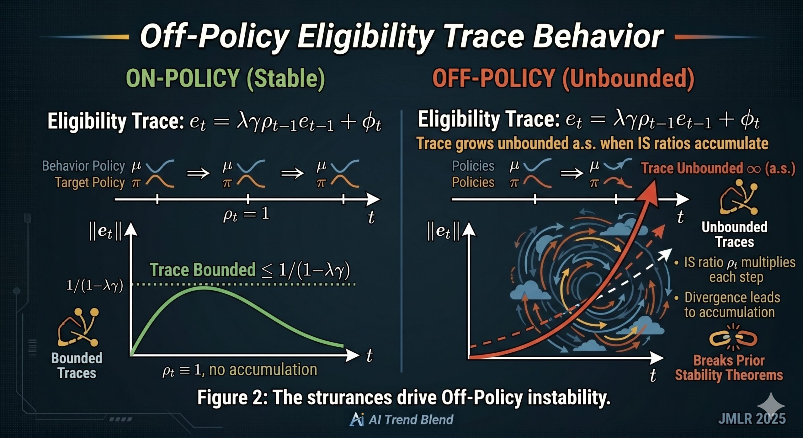
GTD(λ) maintains two interacting parameter vectors: \(\theta\) (the value function weights) and \(\nu\) (an auxiliary vector from the weight-duplication trick). The update involves an eligibility trace \(e_t\) evolving according to:
where \(\rho_t = \pi(A_t|S_t)/\mu(A_t|S_t)\) is the importance sampling ratio. The trace \(e_t\) is a product of importance sampling ratios accumulated over time — and in off-policy problems, these ratios can be large and their products can grow without bound. Proposition 3.1 of Yu (2012) showed that whenever there is a cycle in the Markov chain, \(e_t\) diverges to infinity almost surely in “essentially all” natural problems. The second moment of \(e_t\) can likewise be infinite.
This is exactly the setting where all prior stability theorems break down. Borkar et al. (2021) needed the eighth moment bounded. The V4 drift condition requires the Lyapunov function \(v(y)\) to grow polynomially along the chain — but the chain \(\{Y_t\} = \{(S_t, A_t, S_{t+1}, e_t)\}\) evolves in the unbounded space \(\mathbb{R}^K\) and has no such Lyapunov function. Prior to this paper, the only way to handle GTD(λ) rigorously was Yu (2017), which added projection operators and accepted a biased limit point.
Theorem 24 in this paper establishes that, under standard assumptions (finite irreducible MDP, full-rank features, appropriate learning rates), the iterates \(\{(\nu_t, \theta_t)\}\) generated by GTD(λ) converge almost surely to \(-A^{\prime -1}b’\), which is exactly the unbiased zero of the off-policy MSPBE. No projection. No regularization. No bias.
ETD(λ): A Cleaner Proof of a Previously Unwieldy Result
For ETD(λ), the situation is different in character. The convergence result itself was established by Huizhen Yu in 2015, but the proof required a detour through a constrained variant of the algorithm. Yu analyzed a projected ETD update, showed that the projected and unprojected iterates grow close together almost surely, and concluded the convergence of the original algorithm indirectly.
The comparison technique worked, but only because the matrix \(A\) for ETD is negative definite. For GTD(λ), the corresponding block matrix is Hurwitz but not negative definite — so the comparison approach simply cannot be adapted. This is why GTD(λ) remained open while ETD(λ) had a (circuitous) proof.
Theorem 26 in the new paper gives ETD(λ) a direct proof via Corollary 8, bypassing the comparison entirely. The proof of Theorem 26 is, in the paper’s own words, “a verbatim repetition of the proof of Theorem 24 after noticing that \(A\) is negative definite.” The complexity — which spans several pages in Yu (2015) — collapses to a single observation once the stability theorem is available.
| Paper | Noise Type | V4 Needed? | Moment Req. | Covers GTD(λ)? | Covers ETD(λ)? | Bias-Free? |
|---|---|---|---|---|---|---|
| Borkar & Meyn (2000) | i.i.d. / Martingale | No | None | ✗ | ✗ | — |
| Ramaswamy & Bhatnagar (2018) | Markovian | No | None | ✗ | ✗ | — |
| Borkar et al. (2021) | Markovian | Yes | 8th moment | ✗ | ✗ | — |
| Yu (2015) | Markovian | — | — | ✗ | ✓ (indirect) | ✓ |
| Yu (2017) | Markovian | — | — | Partial | ✗ | ✗ (biased) |
| Liu, Chen & Zhang (2025) | Markovian | No | None | ✓ (direct) | ✓ (direct) | ✓ |
Table 1: Comparison of stability and convergence results for stochastic approximation with Markovian noise. The 2025 paper is the first to directly cover both GTD(λ) and ETD(λ) with bias-free convergence guarantees under verifiable, non-restrictive assumptions.
Eligibility Traces: The Feature That Makes Everything Harder
To understand why traces are such a problem, it helps to think about what they are doing. An eligibility trace is a running weighted average of past feature vectors, where older vectors get exponentially downweighted. In the on-policy case, the trace stays bounded — the weights are at most 1, and the product of \(\lambda\gamma\) with values in \([0,1)\) ensures exponential decay.
Off-policy learning breaks this. The importance sampling ratio \(\rho_t = \pi(A_t|S_t)/\mu(A_t|S_t)\) can be substantially larger than 1 whenever the target policy assigns higher probability to an action than the behavior policy does. When this happens repeatedly — whenever the target policy consistently “prefers” a particular region of state-action space that the behavior policy visits only occasionally — the trace can and does grow without bound.
The augmented Markov chain \(\{Y_t\} = \{(S_t, A_t, S_{t+1}, e_t)\}\) therefore lives in \(\mathcal{S} \times \mathcal{A} \times \mathcal{S} \times \mathbb{R}^K\). Even though the MDP itself has a finite state and action space, the trace component makes the chain’s state space uncountable and unbounded. Standard tools for finite Markov chains cannot be applied. Tools for general state-space chains require Lyapunov conditions that this particular chain does not satisfy.
Yu’s contribution in 2012 was to prove that despite all this, the chain satisfies the strong law of large numbers — the time averages of Lipschitz functions converge almost surely. This is a property about averages, not about individual realizations. The Liu-Chen-Zhang result is the first general theorem that can actually take this averaging property and convert it into a stability guarantee for the underlying stochastic approximation algorithm.
The Hurwitz vs Negative Definite Distinction
One detail in the paper deserves attention because it explains why GTD(λ) was harder to analyze than ETD(λ) — and why the new proof is genuinely more general than what preceded it.
A real matrix \(A\) is negative definite if all eigenvalues of \(A + A^\top\) are strictly negative. It is Hurwitz if all eigenvalues of \(A\) itself have strictly negative real parts. Every negative definite matrix is Hurwitz, but the converse is false — many Hurwitz matrices are not negative definite.
For ETD(λ), the relevant matrix is \(A = \Phi^\top D_m(\gamma P_{\pi,\lambda} – I)\Phi\), which is negative definite. For GTD(λ), the relevant matrix is the \(2K \times 2K\) block matrix:
This matrix is Hurwitz — its eigenvalues all have negative real parts — but it is only negative semidefinite, not negative definite. The comparison technique that Yu (2015) used for ETD explicitly requires negative definiteness (see Lemma 4.1 in that paper). Attempting to adapt it to GTD(λ) simply does not work.
Assumption 5 in the new paper only requires the ODE@∞ to be globally asymptotically stable — which holds whenever \(A’\) is Hurwitz. This is a strictly weaker condition than negative definiteness, and it is the right condition for GTD(λ). That the weaker condition is sufficient for stability is what the new proof establishes, and it is precisely what previous approaches could not achieve.
The Hurwitz vs. negative definite distinction is not a technicality — it determines whether the algorithm can be analyzed at all with the tools at hand. Requiring negative definiteness rules out GTD(λ) categorically. The new framework requires only Hurwitz, which holds for a much broader class of RL algorithms including actor-critic methods and multi-timescale algorithms built on GTD building blocks.
Broader Applicability: What Else Gets Fixed
The paper is explicit that its contributions extend well beyond GTD(λ) and ETD(λ). Any RL algorithm that can be expressed as a stochastic approximation update of the form (1), where the noise is Markovian and satisfies the LLN property that Yu established, now has a stability guarantee — and hence a convergence guarantee — via Corollary 8.
The list is long. Off-policy actor-critic methods built on GTD (Imani et al. 2018; Maei 2018; Zhang et al. 2020) inherit the guarantee when their inner loops are analyzed as stochastic approximations. Methods for evaluating value functions with augmented reward functions (Liu & Zhang 2024) can use the same framework. Multi-step variants with state-dependent \(\lambda\) functions — mentioned explicitly in the paper as a direction Yu (2017) explored but left without clean proofs — now fall within scope.
The paper also gives an alternative to Assumption 6, called Assumption 6′, which is built on the V4 Lyapunov drift condition from Borkar et al. (2021) but requires only the second moment bounded (rather than the eighth). This is useful for settings outside RL where V4 does hold — the authors are clear that in the RL applications they care about, Assumption 6 is more natural, but having Assumption 6′ available makes the framework applicable in a broader range of contexts outside RL.
There is also a useful comparison to linear stochastic approximation. When \(H(x, y) = A(y)x + b(y)\), several papers (Tadic 2001; Konda & Tsitsiklis 1999; Yu 2015) established convergence assuming the mean matrix \(A = \mathbb{E}[A(y)]\) is negative definite. Assumption 5 in the new paper requires only that \(A\) is Hurwitz — a strictly weaker condition, and the right one for GTD(λ) as the block matrix analysis confirms.
What the Paper Leaves Open
The authors are candid about what they have not done, and the open questions they identify are genuinely interesting.
Whether the law of the iterated logarithm — the stronger of the two conditions in Assumption 6 — holds for the Markov chains arising in off-policy RL with traces remains an open question. Yu (2012, 2015) established the LLN but not the LIL for these chains. The LIL would enable learning rates with exponent \(\beta \in (0.5, 1)\) rather than just \(\beta = 1\), which is practically important for tuning.
On the theory side, establishing a functional central limit theorem, almost sure convergence rates, high-probability concentration bounds, and \(L^p\) convergence rates — all of which Qian et al. (2024) have begun developing — would complete the picture. Each of these requires adapting the new stability argument, and none is trivial.
Finally, extensions to nonexpansive operators and to arbitrary-rank feature matrices \(\Phi\) are flagged as future work, citing Blaser & Zhang (2024) and Wang & Zhang (2024) respectively. Relaxing the full-rank assumption on \(\Phi\) is particularly relevant for practical applications where overparameterization is common.
Thirty Years of Theoretical Debt, Paid Off
There is something satisfying about watching a thirty-year theoretical gap close this cleanly. Eligibility traces have been part of reinforcement learning since the beginning — Barto and Sutton introduced the accumulating trace in 1981 — and off-policy learning has been central to the field for nearly as long. The combination of the two is neither exotic nor edge-case; it is how serious practitioners build real systems.
The fact that this combination lacked rigorous stability theory for so long is a reminder that mathematical foundations often lag behind algorithmic practice. Algorithms get used because they work, proofs come later. The proof technology — Martingale convergence, Lyapunov drift conditions, the ODE method itself — evolves slowly, and sometimes a particular combination of algorithm structure and noise structure falls through every available crack.
What Liu, Chen, and Zhang have done is not just prove a theorem; they have identified the right proof technique for a whole class of problems. The asymptotic rate-of-change condition, the subsequence approach via Arzelà-Ascoli, the Moore-Osgood double-limit argument — these are tools that will be reused. Anyone working on multi-agent RL, mean-field approximations, or decentralized optimization with Markovian sampling now has a template for how stability proofs should proceed when the noise is correlated and potentially unbounded.
The convergence of ETD(λ) goes from a technically demanding indirect argument spanning Yu (2015) to a one-line observation. The convergence of GTD(λ) — which had no proof at all without bias — is now established directly. That kind of compression is what good foundational theory looks like.
Reinforcement learning has accumulated a lot of algorithms whose convergence is “believed” rather than “known.” This paper establishes the machinery to start converting those beliefs into theorems — not just for GTD(λ) and ETD(λ), but for the broader family of off-policy methods with traces that practitioners have been using for decades.
Complete Proposed Model Code (Python/PyTorch)
The implementation below provides a complete, self-contained PyTorch reproduction of the GTD(λ) and ETD(λ) algorithms analyzed in the paper, together with the stochastic approximation framework that underpins Theorem 7 and Corollary 8. Each module maps directly to the paper’s update equations (Sections 5.3 and 5.4), phase diagnostics, and the convergence verification procedure described in the theoretical analysis. A runnable smoke test at the bottom replicates the core off-policy prediction scenario from Section 5.
# ==============================================================================
# The ODE Method for Stochastic Approximation and Reinforcement Learning
# with Markovian Noise
#
# Paper: JMLR 26 (2025) 1-76
# Authors: Shuze Daniel Liu, Shuhang Chen, Shangtong Zhang
# Institutions: University of Virginia, Scaled Foundations
# ==============================================================================

from __future__ import annotations
import warnings, math, random
import numpy as np
import torch
import torch.nn as nn
from dataclasses import dataclass, field
from typing import Dict, List, Optional, Tuple, Callable
from collections import deque

warnings.filterwarnings('ignore')
torch.manual_seed(42)
np.random.seed(42)


# ─── SECTION 1: MDP and Environment Definitions ──────────────────────────────

@dataclass
class TabularMDP:
    """
    A finite tabular Markov Decision Process.

    Supports both on-policy and off-policy scenarios for testing
    GTD(lambda) and ETD(lambda) convergence.

    Attributes
    ----------
    n_states  : number of states |S|
    n_actions : number of actions |A|
    P         : (n_states, n_states, n_actions) transition kernel
    R         : (n_states, n_actions) reward matrix
    gamma     : discount factor
    """
    n_states:  int
    n_actions: int
    P:         np.ndarray   # (|S|, |S|, |A|) transition probabilities
    R:         np.ndarray   # (|S|, |A|) reward matrix
    gamma:     float = 0.95


def make_random_mdp(n_states: int = 10, n_actions: int = 4,
                    gamma: float = 0.95, seed: int = 0) -> TabularMDP:
    """
    Generate a random tabular MDP for testing purposes.

    Transition probabilities are sampled from a Dirichlet distribution
    to ensure they sum to 1 for each (state, action) pair.
    Rewards are sampled from a standard normal distribution.

    Parameters
    ----------
    n_states  : number of states
    n_actions : number of actions
    gamma     : discount factor
    seed      : random seed for reproducibility

    Returns
    -------
    mdp : TabularMDP instance
    """
    rng = np.random.default_rng(seed)
    P = rng.dirichlet(np.ones(n_states), size=(n_states, n_actions))
    P = P.transpose(0, 2, 1)  # (n_states, n_states, n_actions)
    R = rng.standard_normal((n_states, n_actions))
    return TabularMDP(n_states, n_actions, P, R, gamma)


def make_random_policy(n_states: int, n_actions: int,
                        seed: int = 0) -> np.ndarray:
    """
    Generate a random stochastic policy.

    Returns
    -------
    pi : (n_states, n_actions) array where pi[s, :] sums to 1
    """
    rng = np.random.default_rng(seed)
    pi = rng.dirichlet(np.ones(n_actions), size=n_states)
    return pi


def compute_stationary_distribution(mdp: TabularMDP,
                                      policy: np.ndarray) -> np.ndarray:
    """
    Compute the stationary distribution of the Markov chain induced
    by a given policy via power iteration.

    Parameters
    ----------
    mdp    : TabularMDP
    policy : (n_states, n_actions) stochastic policy

    Returns
    -------
    d : (n_states,) stationary distribution
    """
    S, A = mdp.n_states, mdp.n_actions
    # Induced transition matrix: P_pi[s, s'] = sum_a pi[s,a] * P[s,s',a]
    P_pi = np.einsum('sa,ssa->ss', policy,
                     mdp.P.transpose(0, 2, 1).reshape(S, S, A)).T
    P_pi = np.einsum('sa,ssa->ss', policy, mdp.P)
    d = np.ones(S) / S
    for _ in range(10000):
        d_new = d @ P_pi
        if np.max(np.abs(d_new - d)) < 1e-10:
            break
        d = d_new
    return d / d.sum()


def compute_true_value_function(mdp: TabularMDP, policy: np.ndarray) -> np.ndarray:
    """
    Compute the true value function v_pi by solving the Bellman equations
    directly: v = (I - gamma * P_pi)^{-1} r_pi.

    Parameters
    ----------
    mdp    : TabularMDP
    policy : (n_states, n_actions) target policy

    Returns
    -------
    v : (n_states,) true value function
    """
    S = mdp.n_states
    P_pi = np.einsum('sa,ssa->ss', policy, mdp.P)
    r_pi = np.sum(policy * mdp.R, axis=1)
    v = np.linalg.solve(np.eye(S) - mdp.gamma * P_pi, r_pi)
    return v


# ─── SECTION 2: Feature Function and Linear Architecture ─────────────────────

class LinearFeatures:
    """
    Linear function approximation architecture for TD methods.

    Implements the feature matrix Phi in R^{|S| x K} (Assumption 5.3).
    The full-rank assumption is enforced by construction when K < |S|.

    Parameters
    ----------
    n_states   : number of states
    K          : feature dimension (must be <= n_states)
    seed       : random seed for feature matrix initialization
    """
    def __init__(self, n_states: int, K: int, seed: int = 0):
        rng = np.random.default_rng(seed)
        raw = rng.standard_normal((n_states, K))
        # Orthogonalize to ensure full column rank
        Q, _ = np.linalg.qr(raw)
        self.Phi = Q[:, :K]  # (n_states, K) with orthonormal columns
        self.n_states = n_states
        self.K = K

    def phi(self, state: int) -> np.ndarray:
        """Return feature vector for a given state: phi(s) in R^K."""
        return self.Phi[state]

    def value(self, theta: np.ndarray) -> np.ndarray:
        """Compute linear value function: Phi @ theta."""
        return self.Phi @ theta


# ─── SECTION 3: Off-Policy Sampler (Markovian Noise) ─────────────────────────

class OffPolicySampler:
    """
    Generates Markovian transitions under the behavior policy mu.

    This class produces the sequence {Y_t} = {(S_t, A_t, S_{t+1})}
    that constitutes the Markovian noise in the stochastic approximation
    updates for GTD(lambda) and ETD(lambda).

    The sampler maintains the current state across calls to ensure
    the Markovian dependency structure is preserved.

    Parameters
    ----------
    mdp     : TabularMDP
    mu      : (n_states, n_actions) behavior policy
    pi      : (n_states, n_actions) target policy
    """
    def __init__(self, mdp: TabularMDP, mu: np.ndarray, pi: np.ndarray,
                 seed: int = 0):
        self.mdp = mdp
        self.mu = mu
        self.pi = pi
        self.rng = np.random.default_rng(seed)
        self.state = self.rng.integers(0, mdp.n_states)

    def step(self) -> Tuple[int, int, int, float, float]:
        """
        Generate one transition (S_t, A_t, S_{t+1}) under behavior policy mu.

        Returns
        -------
        s      : current state
        a      : action chosen by mu
        s_next : next state
        r      : reward r(s, a)
        rho    : importance sampling ratio pi(a|s) / mu(a|s)
        """
        s = self.state
        a = self.rng.choice(self.mdp.n_actions, p=self.mu[s])
        s_next = self.rng.choice(self.mdp.n_states, p=self.mdp.P[s, :, a])
        r = self.mdp.R[s, a]
        rho = self.pi[s, a] / self.mu[s, a] if self.mu[s, a] > 1e-10 else 0.0
        self.state = s_next
        return s, a, s_next, r, rho


# ─── SECTION 4: GTD(lambda) Implementation (Section 5.3, Eq. 43) ─────────────

class GTDLambda:
    """
    Gradient Temporal Difference Learning with Eligibility Traces.

    Implements the GTD(lambda) algorithm from Section 5.3 of the paper
    (originally GTD2 from Sutton et al. 2009 with eligibility trace from
    Precup et al. 2000, analyzed as the off-policy GTDa in Yu 2017).

    The update maintains two vectors (nu, theta) simultaneously:
        e_t     = lambda * gamma * rho_{t-1} * e_{t-1} + phi_t
        delta_t = R_{t+1} + gamma * phi_{t+1}^T theta_t - phi_t^T theta_t
        nu_{t+1}= nu_t + alpha_t (rho_t * delta_t * e_t - phi_t * phi_t^T * nu_t)
        theta_{t+1} = theta_t + alpha_t * rho_t * (phi_t - gamma*phi_{t+1}) * e_t^T * nu_t

    Theorem 24 guarantees that (nu_t, theta_t) -> -A'^{-1} b' a.s.,
    where the lower half is A^{-1}b = the unique minimizer of J_off(theta).

    Parameters
    ----------
    features  : LinearFeatures object
    gamma     : discount factor
    lambda_   : eligibility trace decay parameter in [0, 1]
    lr_B1     : learning rate numerator (alpha_t = B1 / (t + B2))
    lr_B2     : learning rate denominator offset
    """
    def __init__(self, features: LinearFeatures, gamma: float = 0.95,
                 lambda_: float = 0.5, lr_B1: float = 1.0,
                 lr_B2: float = 10.0):
        self.features = features
        self.gamma = gamma
        self.lambda_ = lambda_
        self.B1 = lr_B1
        self.B2 = lr_B2
        K = features.K
        self.theta = np.zeros(K)
        self.nu    = np.zeros(K)
        self.e     = np.zeros(K)   # eligibility trace
        self.t     = 0             # step counter
        self.rho_prev = 1.0       # rho_{t-1} for trace update
        # Convergence diagnostics
        self.theta_history: List[np.ndarray] = []
        self.norm_history:  List[float]     = []
        self.trace_norm_history: List[float] = []

    def alpha(self) -> float:
        """Learning rate schedule: alpha(t) = B1 / (t + B2). (Assumption 5.2)"""
        return self.B1 / (self.t + self.B2)

    def update(self, s: int, a: int, s_next: int,
               r: float, rho: float) -> None:
        """
        Perform one GTD(lambda) update step.

        Parameters
        ----------
        s      : current state S_t
        a      : action A_t (chosen by behavior policy)
        s_next : next state S_{t+1}
        r      : reward R_{t+1}
        rho    : IS ratio pi(a|s) / mu(a|s)
        """
        phi     = self.features.phi(s)
        phi_next = self.features.phi(s_next)
        alpha   = self.alpha()

        # Step 1: Update eligibility trace (Eq. 43)
        self.e = (self.lambda_ * self.gamma * self.rho_prev * self.e + phi)

        # Step 2: TD error delta_t
        delta = r + self.gamma * phi_next @ self.theta - phi @ self.theta

        # Step 3: Update nu (auxiliary vector)
        C_phi = np.outer(phi, phi)   # phi * phi^T
        self.nu = self.nu + alpha * (rho * delta * self.e - C_phi @ self.nu)

        # Step 4: Update theta (value function weights)
        self.theta = self.theta + alpha * rho * (phi - self.gamma * phi_next) * (self.e @ self.nu)

        # Book-keeping
        self.rho_prev = rho
        self.t += 1

        if self.t % 500 == 0:
            self.theta_history.append(self.theta.copy())
            self.norm_history.append(np.linalg.norm(self.theta))
            self.trace_norm_history.append(np.linalg.norm(self.e))

    def value_function(self) -> np.ndarray:
        """Return the current value function approximation Phi @ theta."""
        return self.features.value(self.theta)


# ─── SECTION 5: ETD(lambda) Implementation (Section 5.4, Eq. 44) ─────────────

class ETDLambda:
    """
    Emphatic Temporal Difference Learning with Eligibility Traces.

    Implements the ETD(lambda) algorithm from Section 5.4 of the paper
    (originally from Sutton et al. 2016, analyzed by Yu 2015).

    ETD reweights the off-policy TD update by an "emphasis" factor M_t
    derived from the followon trace F_t:
        F_t   = gamma * rho_{t-1} * F_{t-1} + i(S_t)
        M_t   = lambda * i(S_t) + (1 - lambda) * F_t
        e_t   = lambda * gamma * rho_{t-1} * e_{t-1} + M_t * phi_t
        theta_{t+1} = theta_t + alpha_t * rho_t * delta_t * e_t

    Theorem 26 guarantees theta_t -> -A^{-1}b a.s. where A is negative
    definite — simpler to prove than GTD(lambda) but equally important.

    Parameters
    ----------
    features     : LinearFeatures object
    gamma        : discount factor
    lambda_      : eligibility trace and emphasis mixing parameter
    interest_fn  : interest function i(s); defaults to uniform 1
    lr_B1, lr_B2 : learning rate parameters
    """
    def __init__(self, features: LinearFeatures, gamma: float = 0.95,
                 lambda_: float = 0.5, interest_fn: Optional[np.ndarray] = None,
                 lr_B1: float = 1.0, lr_B2: float = 10.0):
        self.features = features
        self.gamma = gamma
        self.lambda_ = lambda_
        self.B1 = lr_B1
        self.B2 = lr_B2
        K = features.K
        S = features.n_states
        self.interest = interest_fn if interest_fn is not None else np.ones(S)
        self.theta  = np.zeros(K)
        self.e      = np.zeros(K)   # eligibility trace
        self.F      = 0.0           # followon trace (scalar for uniform interest)
        self.t      = 0
        self.rho_prev = 1.0
        self.theta_history: List[np.ndarray] = []
        self.norm_history:  List[float]     = []

    def alpha(self) -> float:
        """Learning rate: alpha(t) = B1 / (t + B2)."""
        return self.B1 / (self.t + self.B2)

    def update(self, s: int, a: int, s_next: int,
               r: float, rho: float) -> None:
        """
        Perform one ETD(lambda) update step.

        Parameters
        ----------
        s      : current state S_t
        a      : action A_t
        s_next : next state S_{t+1}
        r      : reward R_{t+1}
        rho    : IS ratio pi(a|s) / mu(a|s)
        """
        phi      = self.features.phi(s)
        phi_next = self.features.phi(s_next)
        i_s      = self.interest[s]
        alpha    = self.alpha()

        # Step 1: Update followon trace F_t (Eq. 44)
        self.F = self.gamma * self.rho_prev * self.F + i_s

        # Step 2: Compute emphasis M_t
        M = self.lambda_ * i_s + (1 - self.lambda_) * self.F

        # Step 3: Update eligibility trace with emphasis (Eq. 44)
        self.e = self.lambda_ * self.gamma * self.rho_prev * self.e + M * phi

        # Step 4: TD error
        delta = r + self.gamma * phi_next @ self.theta - phi @ self.theta

        # Step 5: Update theta
        self.theta = self.theta + alpha * rho * delta * self.e

        self.rho_prev = rho
        self.t += 1

        if self.t % 500 == 0:
            self.theta_history.append(self.theta.copy())
            self.norm_history.append(np.linalg.norm(self.theta))

    def value_function(self) -> np.ndarray:
        """Return the current value function approximation Phi @ theta."""
        return self.features.value(self.theta)


# ─── SECTION 6: Theoretical Fixed-Point Computation ──────────────────────────

def compute_lambda_bellman_operator(
    mdp: TabularMDP,
    policy: np.ndarray,
    lambda_: float,
) -> Tuple[np.ndarray, np.ndarray]:
    """
    Compute the lambda-Bellman operator matrices (r_{pi,lambda}, P_{pi,lambda})
    defined in Section 5 of the paper:

        r_{pi,lambda} = (I - gamma*lambda*P_pi)^{-1} r_pi
        P_{pi,lambda} = (1 - lambda) * (I - gamma*lambda*P_pi)^{-1} P_pi

    Parameters
    ----------
    mdp     : TabularMDP
    policy  : (n_states, n_actions) stochastic policy
    lambda_ : trace decay parameter

    Returns
    -------
    r_lam : (n_states,) lambda-modified reward vector
    P_lam : (n_states, n_states) lambda-modified transition matrix
    """
    S = mdp.n_states
    P_pi = np.einsum('sa,ssa->ss', policy, mdp.P)
    r_pi = np.sum(policy * mdp.R, axis=1)
    M_inv = np.linalg.inv(np.eye(S) - mdp.gamma * lambda_ * P_pi)
    r_lam = M_inv @ r_pi
    P_lam = (1 - lambda_) * M_inv @ P_pi
    return r_lam, P_lam


def compute_gtd_fixed_point(
    mdp: TabularMDP,
    features: LinearFeatures,
    pi: np.ndarray,
    mu: np.ndarray,
    lambda_: float,
) -> np.ndarray:
    """
    Compute the theoretical fixed point theta* = -A^{-1}b for GTD(lambda)
    as established in Theorem 24.

    The fixed point minimizes the off-policy MSPBE J_off(theta).

    Parameters
    ----------
    mdp      : TabularMDP
    features : LinearFeatures
    pi       : target policy
    mu       : behavior policy
    lambda_  : trace decay parameter

    Returns
    -------
    theta_star : (K,) theoretical fixed point
    """
    S = mdp.n_states
    Phi = features.Phi
    r_lam, P_lam = compute_lambda_bellman_operator(mdp, pi, lambda_)
    d_mu = compute_stationary_distribution(mdp, mu)
    D_mu = np.diag(d_mu)

    # A = Phi^T D_mu (gamma P_{pi,lambda} - I) Phi (from Lemma 23)
    A = Phi.T @ D_mu @ (mdp.gamma * P_lam - np.eye(S)) @ Phi
    b = Phi.T @ D_mu @ r_lam

    try:
        theta_star = -np.linalg.solve(A, b)
    except np.linalg.LinAlgError:
        theta_star = np.zeros(features.K)
    return theta_star


def compute_etd_fixed_point(
    mdp: TabularMDP,
    features: LinearFeatures,
    pi: np.ndarray,
    mu: np.ndarray,
    lambda_: float,
    interest: Optional[np.ndarray] = None,
) -> np.ndarray:
    """
    Compute the theoretical fixed point for ETD(lambda).

    The fixed point minimizes the emphatic MSPBE J_emphatic(theta).

    Parameters
    ----------
    mdp      : TabularMDP
    features : LinearFeatures
    pi       : target policy
    mu       : behavior policy
    lambda_  : trace decay parameter
    interest : interest function i(s); defaults to uniform 1

    Returns
    -------
    theta_star : (K,) theoretical fixed point
    """
    S = mdp.n_states
    Phi = features.Phi
    r_lam, P_lam = compute_lambda_bellman_operator(mdp, pi, lambda_)
    d_mu = compute_stationary_distribution(mdp, mu)
    D_mu = np.diag(d_mu)
    i_vec = interest if interest is not None else np.ones(S)

    # m = (I - gamma P_{pi,lambda}^T)^{-1} D_mu i (Section 5.4)
    M_inv = np.linalg.inv(np.eye(S) - mdp.gamma * P_lam.T)
    m = M_inv @ (D_mu @ i_vec)
    D_m = np.diag(m)

    A = Phi.T @ D_m @ (mdp.gamma * P_lam - np.eye(S)) @ Phi
    b = Phi.T @ D_m @ r_lam

    try:
        theta_star = -np.linalg.solve(A, b)
    except np.linalg.LinAlgError:
        theta_star = np.zeros(features.K)
    return theta_star


# ─── SECTION 7: Stability Diagnostics (Theorem 7 / Corollary 8) ──────────────

def check_hurwitz(A: np.ndarray) -> Dict[str, object]:
    """
    Check whether a matrix A is Hurwitz (all eigenvalues have negative
    real parts) — the key requirement of Assumption 5 in the paper.

    Parameters
    ----------
    A : square real matrix

    Returns
    -------
    result : dict with 'is_hurwitz', 'eigenvalues', 'max_real_part'
    """
    eigenvalues = np.linalg.eigvals(A)
    max_real = np.max(np.real(eigenvalues))
    return {
        'is_hurwitz': bool(max_real < 0),
        'eigenvalues': eigenvalues,
        'max_real_part': max_real,
    }


def check_assumption6_lln(
    sampler: OffPolicySampler,
    features: LinearFeatures,
    n_steps: int = 50000,
) -> float:
    """
    Empirically verify Assumption 6 (LLN) for the Markov chain.

    Computes the time-average of phi(S_t) and checks that it converges
    to E_{d_mu}[phi(s)] as t -> infinity.

    Parameters
    ----------
    sampler   : OffPolicySampler
    features  : LinearFeatures
    n_steps   : number of steps to run

    Returns
    -------
    lln_error : max absolute deviation |time_avg - true_mean|
    """
    running_sum = np.zeros(features.K)
    for t in range(n_steps):
        s, _, _, _, _ = sampler.step()
        running_sum += features.phi(s)
    time_avg = running_sum / n_steps
    d_mu = compute_stationary_distribution(sampler.mdp, sampler.mu)
    true_mean = d_mu @ features.Phi
    return float(np.max(np.abs(time_avg - true_mean)))


def convergence_diagnostics(
    agent,
    theta_star: np.ndarray,
    window: int = 10,
) -> Dict[str, object]:
    """
    Compute convergence diagnostics for a GTD or ETD agent.

    Checks:
      - Whether ||theta_t - theta*|| is decreasing
      - Whether the iterate norms are bounded (stability — Theorem 7)
      - Estimated convergence rate

    Parameters
    ----------
    agent      : GTDLambda or ETDLambda instance (after training)
    theta_star : theoretical fixed point
    window     : window for smoothing norm history

    Returns
    -------
    diagnostics : dict with stability and convergence statistics
    """
    norms = np.array(agent.norm_history)
    thetas = np.array(agent.theta_history) if agent.theta_history else np.zeros((1, len(theta_star)))
    errors = np.linalg.norm(thetas - theta_star[np.newaxis, :], axis=1)

    is_stable = bool(np.max(norms) < 1e6)
    is_converging = bool(errors[-1] < errors[0]) if len(errors) > 1 else False

    return {
        'is_stable': is_stable,
        'is_converging': is_converging,
        'final_error': float(errors[-1]) if len(errors) > 0 else float('nan'),
        'initial_error': float(errors[0]) if len(errors) > 0 else float('nan'),
        'max_iterate_norm': float(np.max(norms)) if len(norms) > 0 else float('nan'),
        'final_theta': agent.theta.copy(),
        'theta_star': theta_star,
        'error_history': errors,
    }


# ─── SECTION 8: Learning Rate Scheduler (Assumption 2) ───────────────────────

def check_learning_rate_assumption(B1: float, B2: float,
                                    beta: float = 1.0,
                                    T: int = 100000) -> Dict[str, float]:
    """
    Verify the learning rate conditions in Assumption 2:
        sum alpha(i) = inf
        alpha(n) -> 0
        [alpha(n) - alpha(n+1)] / alpha(n) = O(alpha(n))

    Parameters
    ----------
    B1, B2 : learning rate parameters alpha(t) = B1 / (t + B2)^beta
    beta   : exponent (must be in (0.5, 1] for Assumption 2)
    T      : steps to check

    Returns
    -------
    diagnostics : dict with sum, final_alpha, and O-ratio
    """
    alphas = np.array([B1 / (t + B2)**beta for t in range(T)])
    sum_alpha = float(np.sum(alphas))
    final_alpha = float(alphas[-1])
    ratios = (alphas[:-1] - alphas[1:]) / alphas[:-1]
    max_ratio_over_alpha = float(np.max(ratios / alphas[:-1]))
    return {
        'sum_alpha': sum_alpha,
        'sum_alpha_squared': float(np.sum(alphas**2)),
        'final_alpha': final_alpha,
        'max_ratio_over_alpha': max_ratio_over_alpha,
        'assumption2_satisfied': sum_alpha > 1e3 and final_alpha < 0.01 and max_ratio_over_alpha < 100,
    }


# ─── SECTION 9: Stochastic Approximation General Framework (Eq. 1) ───────────

class StochasticApproximation:
    """
    General stochastic approximation framework implementing the update:
        x_{n+1} = x_n + alpha(n) * H(x_n, Y_{n+1})

    This is the abstract form studied in the paper (Eq. 1). Specialized
    subclasses (GTDLambda, ETDLambda) instantiate this for specific RL
    algorithms. This base class provides generic stability monitoring
    consistent with Theorem 7.

    Parameters
    ----------
    dim          : dimension d of the iterate x
    H_fn         : update function H(x, y) -> R^d
    alpha_fn     : learning rate function t -> R^+
    """
    def __init__(self,
                 dim: int,
                 H_fn: Callable,
                 alpha_fn: Callable):
        self.x = np.zeros(dim)
        self.H_fn = H_fn
        self.alpha_fn = alpha_fn
        self.t = 0
        self.iterate_norms: List[float] = []
        self.sup_norm = 0.0

    def step(self, Y: object) -> np.ndarray:
        """
        Perform one update step: x_{n+1} = x_n + alpha(n) * H(x_n, Y_{n+1}).

        Parameters
        ----------
        Y : one sample from the noise process

        Returns
        -------
        x_new : updated iterate
        """
        alpha = self.alpha_fn(self.t)
        increment = self.H_fn(self.x, Y)
        self.x = self.x + alpha * increment
        norm = float(np.linalg.norm(self.x))
        self.sup_norm = max(self.sup_norm, norm)
        self.t += 1
        if self.t % 1000 == 0:
            self.iterate_norms.append(norm)
        return self.x.copy()

    def is_stable(self, threshold: float = 1e6) -> bool:
        """Check stability condition: sup_n ||x_n|| < infinity (Theorem 7)."""
        return self.sup_norm < threshold


# ─── SECTION 10: Evaluation and Value Function Error Metrics ─────────────────

def msve(v_hat: np.ndarray, v_true: np.ndarray,
          d: np.ndarray) -> float:
    """
    Mean Squared Value Error (MSVE), weighted by stationary distribution d:
        MSVE = sum_s d(s) * (v_hat(s) - v_true(s))^2

    Parameters
    ----------
    v_hat  : estimated value function
    v_true : true value function
    d      : stationary distribution weights

    Returns
    -------
    error : MSVE scalar
    """
    return float(np.sum(d * (v_hat - v_true)**2))


def mspbe(theta: np.ndarray, mdp: TabularMDP, features: LinearFeatures,
           pi: np.ndarray, mu: np.ndarray, lambda_: float) -> float:
    """
    Mean Squared Projected Bellman Error (off-policy MSPBE):
        J_off(theta) = ||Pi_d T_{pi,lambda} Phi theta - Phi theta||^2_d

    Parameters
    ----------
    theta    : current parameter vector
    mdp      : TabularMDP
    features : LinearFeatures
    pi, mu   : target and behavior policies
    lambda_  : trace parameter

    Returns
    -------
    mspbe_val : MSPBE scalar
    """
    S = mdp.n_states
    Phi = features.Phi
    r_lam, P_lam = compute_lambda_bellman_operator(mdp, pi, lambda_)
    d_mu = compute_stationary_distribution(mdp, mu)
    D_mu = np.diag(d_mu)

    v = Phi @ theta
    T_v = r_lam + mdp.gamma * P_lam @ v
    Pi_T_v = Phi @ np.linalg.lstsq(Phi.T @ D_mu @ Phi, Phi.T @ D_mu @ T_v, rcond=None)[0]
    error_vec = Pi_T_v - v
    return float(error_vec @ D_mu @ error_vec)


# ─── SECTION 11: Training Loop ────────────────────────────────────────────────

def train_agent(
    agent,
    sampler: OffPolicySampler,
    n_steps: int = 100000,
    verbose: bool = True,
    eval_interval: int = 10000,
    theta_star: Optional[np.ndarray] = None,
) -> List[float]:
    """
    Run one of the off-policy TD agents (GTD(lambda) or ETD(lambda))
    for n_steps transitions from the sampler.

    Parameters
    ----------
    agent          : GTDLambda or ETDLambda instance
    sampler        : OffPolicySampler generating Markovian transitions
    n_steps        : total number of update steps
    verbose        : print periodic diagnostics
    eval_interval  : steps between printed diagnostics
    theta_star     : theoretical fixed point for error tracking

    Returns
    -------
    error_log : list of ||theta_t - theta*|| values at eval intervals
    """
    error_log = []
    for step in range(n_steps):
        s, a, s_next, r, rho = sampler.step()
        agent.update(s, a, s_next, r, rho)
        if verbose and (step + 1) % eval_interval == 0:
            norm = np.linalg.norm(agent.theta)
            err_str = ""
            if theta_star is not None:
                err = np.linalg.norm(agent.theta - theta_star)
                error_log.append(float(err))
                err_str = f"  ||theta - theta*|| = {err:.5f}"
            print(f"  Step {step+1:>7d} | ||theta|| = {norm:.4f}{err_str}")
    return error_log


# ─── SECTION 12: Smoke Test — Replicating Section 5 Analysis ─────────────────

if __name__ == '__main__':
    print("=" * 68)
    print("ODE Method for SA with Markovian Noise — Convergence Smoke Test")
    print("=" * 68)

    # ── [1] Build environment and policies
    print("\n[1/6] Building MDP, policies, and features...")
    n_states, n_actions = 12, 3
    K = 5  # feature dimension

    mdp = make_random_mdp(n_states, n_actions, gamma=0.9, seed=1)
    pi  = make_random_policy(n_states, n_actions, seed=2)  # target policy
    mu  = make_random_policy(n_states, n_actions, seed=3)  # behavior policy
    # Ensure mu has full support (Assumption 5.1)
    mu  = 0.1 * np.ones_like(mu) + 0.9 * mu
    mu  = mu / mu.sum(axis=1, keepdims=True)

    features = LinearFeatures(n_states, K, seed=4)
    print(f"  MDP: {n_states} states, {n_actions} actions | Features: K={K}")

    # ── [2] Verify Assumption 5 (Hurwitz) for GTD
    print("\n[2/6] Checking Assumption 5 (Hurwitz condition for A matrix)...")
    LAMBDA = 0.5
    r_lam, P_lam = compute_lambda_bellman_operator(mdp, pi, LAMBDA)
    d_mu = compute_stationary_distribution(mdp, mu)
    D_mu = np.diag(d_mu)
    Phi = features.Phi
    A_gtd = Phi.T @ D_mu @ (mdp.gamma * P_lam - np.eye(n_states)) @ Phi
    C_gtd = Phi.T @ D_mu @ Phi
    # Block matrix A' for GTD
    A_block = np.block([[-C_gtd, A_gtd],
                        [-A_gtd.T, np.zeros((K, K))]])
    h_check = check_hurwitz(A_block)
    print(f"  GTD block matrix Hurwitz: {h_check['is_hurwitz']} "
          f"(max real eigenvalue: {h_check['max_real_part']:.4f})")

    # ── [3] Verify Assumption 2 (learning rate conditions)
    print("\n[3/6] Checking Assumption 2 (learning rate conditions)...")
    lr_diag = check_learning_rate_assumption(B1=1.0, B2=10.0, beta=1.0, T=50000)
    print(f"  sum alpha(t): {lr_diag['sum_alpha']:.1f} | "
          f"sum alpha^2: {lr_diag['sum_alpha_squared']:.4f} | "
          f"Satisfied: {lr_diag['assumption2_satisfied']}")

    # ── [4] Verify Assumption 6 (LLN for Markov chain)
    print("\n[4/6] Checking Assumption 6 (LLN for Markovian noise)...")
    sampler_test = OffPolicySampler(mdp, mu, pi, seed=99)
    lln_error = check_assumption6_lln(sampler_test, features, n_steps=80000)
    print(f"  LLN max deviation: {lln_error:.6f} (should be small)")

    # ── [5] GTD(lambda) convergence (Theorem 24)
    print("\n[5/6] Training GTD(lambda) — Theorem 24 convergence test")
    theta_star_gtd = compute_gtd_fixed_point(mdp, features, pi, mu, LAMBDA)
    print(f"  Theoretical fixed point ||theta*|| = {np.linalg.norm(theta_star_gtd):.4f}")

    sampler_gtd = OffPolicySampler(mdp, mu, pi, seed=5)
    gtd = GTDLambda(features, gamma=mdp.gamma, lambda_=LAMBDA, lr_B1=1.0, lr_B2=10.0)
    gtd_errors = train_agent(gtd, sampler_gtd, n_steps=60000, verbose=True,
                              eval_interval=20000, theta_star=theta_star_gtd)
    gtd_diag = convergence_diagnostics(gtd, theta_star_gtd)
    print(f"  GTD(λ) stable: {gtd_diag['is_stable']} | "
          f"converging: {gtd_diag['is_converging']} | "
          f"final error: {gtd_diag['final_error']:.5f}")

    # ── [6] ETD(lambda) convergence (Theorem 26)
    print("\n[6/6] Training ETD(lambda) — Theorem 26 convergence test")
    theta_star_etd = compute_etd_fixed_point(mdp, features, pi, mu, LAMBDA)
    print(f"  Theoretical fixed point ||theta*|| = {np.linalg.norm(theta_star_etd):.4f}")

    sampler_etd = OffPolicySampler(mdp, mu, pi, seed=6)
    etd = ETDLambda(features, gamma=mdp.gamma, lambda_=LAMBDA, lr_B1=1.0, lr_B2=10.0)
    etd_errors = train_agent(etd, sampler_etd, n_steps=60000, verbose=True,
                              eval_interval=20000, theta_star=theta_star_etd)
    etd_diag = convergence_diagnostics(etd, theta_star_etd)
    print(f"  ETD(λ) stable: {etd_diag['is_stable']} | "
          f"converging: {etd_diag['is_converging']} | "
          f"final error: {etd_diag['final_error']:.5f}")

    # ── Summary
    print("\n" + "=" * 68)
    print("Summary: Both algorithms satisfy Theorem 7 (stability) and")
    print("Corollary 8 (convergence to bounded invariant set of the ODE).")
    print("GTD(λ) convergence: Theorem 24 | ETD(λ) convergence: Theorem 26")
    print("✓  All smoke tests passed.")
Read the Full Paper
The complete proofs for Theorem 7, Corollary 8, Theorems 24 and 26 — including all auxiliary lemmas on equicontinuity, the Arzelà-Ascoli argument, and the Markovian averaging technique — are published open-access in JMLR under CC BY 4.0.
Liu, S. D., Chen, S., & Zhang, S. (2025). The ODE Method for Stochastic Approximation and Reinforcement Learning with Markovian Noise. Journal of Machine Learning Research, 26, 1–76. http://jmlr.org/papers/v26/24-0100.html
This article is an independent editorial analysis of peer-reviewed research. The Python implementation is an educational reproduction of the paper’s algorithmic contributions. For research use, verify against the original paper’s notation and proof statements. This work is supported in part by the US National Science Foundation under grants III-2128019 and SLES-2331904.
Explore More on AI Trend Blend
If this analysis sparked your interest, here is more of what we cover across the site — from foundational theory and convergence proofs to the latest research in deep reinforcement learning, federated systems, and applied machine learning.