
This article explains a published research paper. It is not medical advice, diagnosis, or treatment guidance. The segmentation model discussed here is a research prototype, not an approved clinical device. Anyone with a health concern about a breast finding should speak with a qualified radiologist or physician.
Key points
- Researchers found and corrected duplicate images inside the widely used BUSI breast ultrasound dataset, which had been inflating reported segmentation scores through data leakage between training and validation sets.
- A modified Residual Encoder U-Net trained with the nnU-Net framework reached a Dice score of 0.7726 on in domain validation on the Breast-Lesion-USG dataset, ahead of ResUNet, UNet++, Attention-UNet, SwinUNet, and a diffusion based baseline called D-DDPM.
- The same model, trained on the deduplicated BUSI-A3 subset and tested on a different hospital’s scanner and population, dropped to a Dice score of 0.4855, a collapse of roughly 37 percent.
- Three epistemic uncertainty methods were compared. Monte Carlo dropout, deep ensembles, and a combined approach, all evaluated across 83 million analyzed pixels from 256 cases.
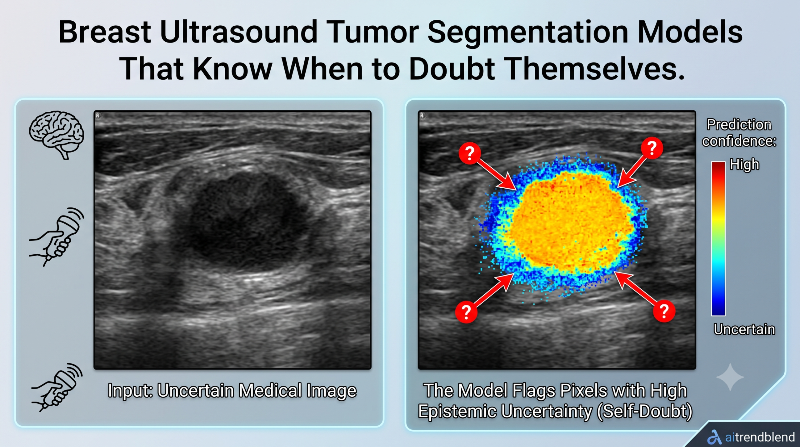
- Higher predictive entropy and mutual information tracked the accuracy collapse under domain shift, giving a practical signal for when a prediction should be treated with suspicion.
The dataset everyone uses has a leak
If you have spent any time reading breast ultrasound segmentation papers, you have run into the BUSI dataset. Al Dhabyani and colleagues released it in 2020, and it became something close to a default benchmark for the field. Grayscale images, binary masks, three classes covering normal, benign, and malignant tissue. Convenient, public, and widely cited.
The problem is that BUSI is not as clean as its popularity implies. A 2023 correction by Pawłowska, Karwat, and Żołek flagged duplicated images inside the set, and this new paper goes further. The authors report that the duplicated pairs often carried different annotations, meaning the same underlying scan could show up twice with two different radiologists drawing two different boundaries around the same lesion. Worse, some of what shipped inside a breast ultrasound dataset was not breast tissue at all. The paper notes an inadvertent inclusion of maxilla ultrasound images, jaw scans that have no business being scored alongside breast tumor masks.
Why does this matter beyond dataset hygiene? Because when a duplicate scan lands in the training split and its twin lands in the validation split, a model does not need to generalize to score well. It just needs to recognize a picture it has already memorized. That is data leakage, and it quietly inflates every metric downstream. A model can look like it segments tumors well while actually segmenting a handful of images it has seen twice.
The team’s response was methodical rather than dramatic. They built three deduplicated variants of BUSI. BUSI-A1 removes the first occurrence of each duplicate pair. BUSI-A2 removes the second occurrence. BUSI-A3 keeps whichever version of the duplicate a trained radiologist judged to be the more accurate annotation. Three different philosophies for handling the same underlying mess, which lets the paper show how much the choice of cleanup strategy actually moves the needle, rather than asserting one fix and hoping it is representative.
Why this matters
Any published Dice score on the raw BUSI dataset should now be read with a healthy dose of skepticism. If a paper reports strong numbers on BUSI without mentioning deduplication, there is a real chance those numbers are propped up by leakage rather than genuine segmentation skill.
A residual encoder built for stability, not novelty
The architecture itself is deliberately unglamorous. Instead of chasing a new attention mechanism or a diffusion backbone, the authors built a modified Residual Encoder U-Net and trained it with the nnU-Net framework, the self configuring segmentation pipeline that Isensee and colleagues have continued to refine. This is a practical choice. nnU-Net has a track record of squeezing strong performance out of relatively standard architectures by getting the preprocessing, patch size, and training schedule right rather than reinventing the network.
The encoder runs eight stages deep, paired with seven decoder stages, each one widening the feature maps as the spatial resolution shrinks. The residual block at the center of each stage follows a specific six layer pattern. A convolution feeds into dropout, then instance normalization, then a leaky ReLU activation, then a second convolution, then a second instance normalization. That dropout layer sitting inside the residual block is not incidental. It is the same mechanism the paper later reuses at inference time to estimate uncertainty, so the architecture and the uncertainty method are built around the same switch rather than bolted together as separate systems.
Training details are concrete rather than vague. Patches of 512 by 512 pixels, a batch size of 13, stochastic gradient descent, a batch dice loss, and deep supervision so that intermediate decoder stages also receive gradient signal rather than only the final output layer. Every fold trains for 250 epochs by default. The BUSI-A3 variant, which the team ultimately recommends as the most trustworthy deduplication strategy, gets an additional 750 epochs, a full 1000 epochs total, before it is used for the out of distribution evaluation. That extra training budget for the model that matters most for the paper’s central claim is a small but telling detail. It suggests the authors wanted their out of distribution numbers to reflect a genuinely converged model rather than an undertrained one that might exaggerate the domain shift problem.
The residual block transformation for input tensor \(x\) with weights \(\theta\) can be written as
$$ y = \text{LeakyReLU}\Big(\text{IN}\big(\text{Conv}_2(\text{IN}(\text{Dropout}(\text{Conv}_1(x))))\big) + \text{skip}(x)\Big) $$where IN denotes instance normalization and skip is an identity mapping or a projection when the channel count or stride changes between the input and the block output.
Two test sets, two very different jobs
A second dataset does the heavy lifting for evaluating whether any of this generalizes. Breast-Lesion-USG, curated by Pawłowska and colleagues and published in Scientific Data in 2024, serves two purposes here. First, the team runs a full five fold cross validation directly on Breast-Lesion-USG to establish an in domain benchmark, essentially asking how well the architecture performs when trained and tested on the same distribution. Second, in the setup that matters most for this story, they take the model trained only on BUSI-A3 and test it cold on Breast-Lesion-USG, with zero fine tuning on the target hospital’s data. That second setup is the out of distribution test, and it is where the real story of this paper lives.
The in domain numbers look good
Table 1 in the paper reports five fold Dice scores across the four BUSI variants. BUSI-Full, the uncleaned dataset with duplicates intact, posts an average Dice of 0.7514. The three deduplicated variants come in lower. BUSI-A1 averages 0.7144, BUSI-A2 averages 0.7179, and BUSI-A3 averages 0.7211. That gap between the full dataset and every cleaned version is not noise. It is the leakage effect made visible in a single table. Once the duplicate pairs are removed and a model can no longer partially memorize its validation set, its apparent performance drops by roughly three Dice points across the board.
On the Breast-Lesion-USG benchmark, trained and validated on the same distribution with five fold cross validation over 250 epochs, the model reaches an average Dice score of 0.7726 with a standard deviation of 0.0212. Table 2 lines this up against other published methods evaluated on the same dataset. ResUNet manages a Dice of 0.4563 and an IoU of 0.3444. UNet++ comes in at 0.3734 and 0.2564. Attention-UNet reaches 0.4764 and 0.3000. SwinUNet, the transformer based entry, sits at 0.4436 and 0.3331. A diffusion model approach called D-DDPM does considerably better, at 0.7104 and 0.6140. The paper’s own benchmark result, 0.7726 Dice and 0.6801 IoU, edges out all of them, including the diffusion baseline.
| Model | Dice | IoU |
|---|---|---|
| ResUNet | 0.4563 | 0.3444 |
| UNet++ | 0.3734 | 0.2564 |
| Attention-UNet | 0.4764 | 0.3000 |
| SwinUNet | 0.4436 | 0.3331 |
| D-DDPM | 0.7104 | 0.6140 |
| Ours, in domain benchmark | 0.7726 | 0.6801 |
| Ours, BUSI-A3 trained, out of distribution | 0.4855 | 0.4309 |
Taken alone, that in domain result is the kind of number that gets a paper accepted and gets a model quietly deployed somewhere. It would be easy to stop the story there. The authors do not stop there, and that decision is the most important thing about this work.
The out of distribution number is the real headline
Here is where it gets interesting. Take the model trained on BUSI-A3, the radiologist curated, deduplicated subset, and point it at Breast-Lesion-USG with no fine tuning. The Dice score falls to 0.4855 and the IoU falls to 0.4309, shown in the bottom row of Table 2. Against the in domain benchmark of 0.7726 Dice, that is a drop of almost 0.29 Dice points, a relative collapse of roughly 37 percent. Notice also where that out of distribution number lands relative to the other methods in Table 2. At 0.4855 Dice, the same architecture that topped the leaderboard when trained and tested on matching data now performs in the same range as ResUNet, UNet++, and SwinUNet, methods it had just outperformed by a wide margin. The architecture did not get worse. The distribution shifted, different scanners, different patient populations, different acquisition protocols, and the model’s apparent skill mostly evaporated with it.
This is not a new phenomenon in medical imaging research, domain shift has been a known problem for years, but the size of the gap here is worth sitting with. A model that looks state of the art on paper can behave like a much weaker baseline the moment it meets a hospital it was not trained on. Anyone evaluating a segmentation tool for real deployment, not just for a leaderboard entry, needs a way to know when they have crossed into that weaker territory. That is exactly the gap the uncertainty estimation work is built to fill.
Three ways to ask a model how sure it is
Epistemic uncertainty, the flavor of uncertainty that comes from what the model has not learned rather than from inherent noise in the image, can be estimated without retraining an entirely new kind of network. The paper compares three approaches, all applied to the same underlying architecture.
Monte Carlo dropout
The dropout layers sitting inside those residual blocks are normally switched off at inference time. Monte Carlo dropout keeps them active. Run the same input through the network multiple times with dropout still randomly zeroing out activations, and each pass produces a slightly different prediction because a slightly different subnetwork answered the question. Average those predictions for the final output, and use the spread across passes as a proxy for how uncertain the model is. The paper runs ten stochastic forward passes per case.
where \(f_{\theta_t}(x)\) is the prediction produced at stochastic pass \(t\) with a different random subset of weights dropped, and \(T\) is the total number of passes, ten in this study.
Deep ensembles
A more expensive but often more informative approach trains several full models independently, with different random initializations and data ordering, then averages their predictions. Disagreement among genuinely separate models tends to capture a different and often larger slice of epistemic uncertainty than dropout sampling alone, since it reflects variability from the training process itself rather than just from a single trained network being perturbed at test time.
where each \(\theta^{(k)}\) represents an independently trained ensemble member, with \(K\) members contributing to the averaged prediction.
The combined approach
The paper also tries stacking both methods, running each of five ensemble members through three stochastic dropout passes apiece, for fifteen total samples per case. This jointly captures both the disagreement between separately trained models and the internal uncertainty each of those models expresses about its own prediction.
Aleatoric uncertainty, the kind that comes from inherent sensor noise or ambiguous anatomy rather than from limits on what the model has learned, is not modeled by any of these three methods. That is a scope choice the authors state plainly rather than a gap they overlook.
Measuring confidence at the pixel level
None of these methods matter unless the resulting uncertainty is actually measured and checked for whether it lines up with reality. The paper leans on three pixel level metrics across all 256 cases of the Breast-Lesion-USG dataset, spanning 83,099,921 analyzed pixels, including roughly 5.8 million foreground pixels that actually belong to a lesion.
Predictive entropy captures total uncertainty at each pixel by looking at how close the averaged probability sits to the uncertain midpoint of 0.5 rather than confidently near 0 or 1.
where \(\bar{p}_{ij}\) is the mean predicted probability at pixel position \((i,j)\) averaged across the \(T\) stochastic forward passes.
Mutual information isolates the epistemic component specifically, subtracting out the average entropy of the individual passes from the entropy of the averaged prediction. What remains is the disagreement between passes, which is what the model does not know, as opposed to what looks inherently blurry in the image regardless of which version of the model is asked.
Expected calibration error checks whether stated confidence and actual correctness line up. Pixels get sorted into 30 confidence bins, and for each bin the paper compares average predicted confidence against the actual accuracy of pixels that fell into that bin.
where \(B_m\) is a confidence bin, \(N\) is the total pixel count, and lower values indicate that the model’s stated confidence is closer to how often it is actually correct.
What the uncertainty numbers actually show
Table 3 lays out the comparison across all three uncertainty methods, and the pattern is worth walking through carefully because it runs slightly against a naive intuition that more sophisticated methods should always report higher uncertainty.
| Method | Entropy | Mutual information | ECE | Pixel accuracy |
|---|---|---|---|---|
| Monte Carlo dropout | 0.009 | 0.002 | 0.0367 | 0.9595 |
| Deep ensemble | 0.021 | 0.013 | 0.0300 | 0.9607 |
| Deep ensemble plus MC dropout | 0.031 | 0.019 | 0.0303 | 0.9604 |
Monte Carlo dropout alone produced the lowest average entropy at 0.009 and the lowest average mutual information at 0.002, with a range stretching from 0.000 up to 0.693 for entropy and up to 0.488 for mutual information. The median values across cases sat near zero for both metrics, which tells you that on a typical pixel, the ten stochastic passes mostly agreed with each other. Deep ensembles reported noticeably higher uncertainty, a mean entropy of 0.021 and mean mutual information of 0.013, with wider standard deviations too, 0.076 for entropy compared to 0.046 for MC dropout. Independently trained models disagree with each other more than the same model perturbed by dropout disagrees with itself, which lines up with what a lot of uncertainty quantification research has found in other domains. The combined approach pushed uncertainty higher still, to 0.031 mean entropy and 0.019 mean mutual information, consistent with it drawing on both sources of variability at once.
Calibration told a slightly different story. Deep ensembles and the combined approach both beat plain Monte Carlo dropout on expected calibration error, 0.0300 and 0.0303 respectively against 0.0367 for MC dropout alone, and both also edged out MC dropout on raw pixel accuracy. So while MC dropout reports the smallest uncertainty numbers, it is also the least well calibrated of the three, meaning its confidence scores track its actual correctness slightly less faithfully than the ensemble based methods do.
A caution worth keeping in mind
Pixel accuracy above 0.95 for every method looks reassuring at first glance, but the paper is upfront that this figure is inflated by the sheer imbalance between background and foreground pixels. With only about 5.8 million of the 83 million analyzed pixels belonging to a lesion, a model could in principle score high accuracy by being conservative about background while still missing meaningful tumor area. Dice and IoU, which weight the foreground region more heavily, remain the more trustworthy segmentation metrics here.
Clinical translation gap
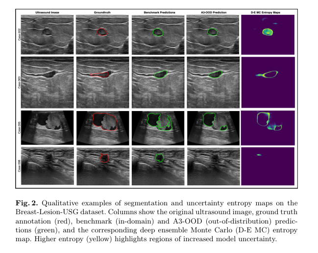
There is a meaningful distance between what happens in this study and what would need to happen for a tool like this to sit inside an actual breast imaging workflow. The out of distribution collapse, from a Dice score near 0.77 down to roughly 0.49, is measured against exactly one target dataset, Breast-Lesion-USG, drawn from a specific set of scanners and a specific patient population in Poland. A hospital in a different country, using different ultrasound equipment and scanning a population with different breast density distributions, could see a different pattern of failure entirely. The uncertainty maps are a genuinely useful signal, higher entropy did track lower accuracy under domain shift in this study, but nothing here has been tested in an actual clinical reading workflow where a radiologist would need to decide, in real time, how much weight to give a confidence overlay next to their own judgment. The paper also notes that Monte Carlo dropout and deep ensembles increase inference time by 10 to 25 times compared with a single forward pass, which is a real constraint for any setting where scan volume is high and turnaround time matters.
Honest limitations
The authors are candid about where this work stops short. Expected calibration error depends on the binning scheme used to compute it, and the paper notes this can be sensitive and may not generalize cleanly across different data distributions. Pixel wise accuracy, as already discussed, is inflated by the imbalance between foreground and background pixels in a typical ultrasound frame, where the actual lesion usually occupies a small fraction of the image.
Clinical limitations
Sample size is a genuine constraint here. The out of distribution evaluation draws on 256 cases from Breast-Lesion-USG, which is a reasonable size for a research benchmark but small relative to the population diversity a deployed tool would eventually meet. Dataset bias is baked into both source datasets, BUSI and Breast-Lesion-USG each reflect the equipment, protocols, and patient demographics of the specific clinical sites where they were collected, and neither claims to represent breast tissue presentation globally. Generalization, as the out of distribution results make plain, cannot be assumed even between two public benchmark datasets that both claim to represent breast ultrasound imaging. The paper itself frames this as a call for future adaptive models and further calibration research rather than as a finished solution, and readers should take that framing at face value.
Where this could go next
The most interesting suggestion buried in the discussion section has nothing to do with model architecture. BUSI-Full, before deduplication, contains multiple annotator segmentations for some cases, meaning more than one radiologist drew a boundary for the same lesion. The authors point out that this kind of data, collected with intentional design rather than as an accidental byproduct of dataset assembly, could let a model’s uncertainty calibration be checked against genuine clinical disagreement rather than only against a single majority vote mask. Two radiologists disagreeing about where a boundary sits is itself a form of ground truth uncertainty, and a model that is well calibrated should ideally express more uncertainty in exactly the regions where human experts also disagree.
That is a meaningfully different research direction from simply scaling up ensemble size or trying a fancier backbone. It treats human disagreement as a signal worth modeling rather than as noise to average away, and it would require datasets built from the ground up with that goal in mind rather than assembled after the fact.
The bigger picture for anyone building on public medical datasets
Step back from the specific numbers and there is a broader lesson here for anyone working with public medical imaging benchmarks generally, not just breast ultrasound. Popular datasets get reused for years, papers cite each other’s reported scores without necessarily auditing the underlying data again, and small integrity problems like duplicate images can persist quietly in a field’s shared benchmark for a long time before anyone traces a performance drop back to a data cleaning issue rather than an architecture choice.
The correction effort here, catching and quantifying leakage inside BUSI, mirrors similar cleanup work that has surfaced in other medical imaging benchmarks over the past several years. It is not a flashy contribution compared to a new segmentation architecture, but arguably it matters more, since every architecture paper that trains on the uncleaned version of a leaky dataset inherits an inflated sense of its own performance. Pairing that kind of dataset audit with an uncertainty estimation framework that actually gets validated against a genuine out of distribution test, rather than only against a held out split of the same dataset, is a combination that more medical imaging papers could stand to adopt.
Takeaway for practitioners
If you are evaluating or deploying a segmentation model trained on a public benchmark, treat any reported Dice score with a question attached. Was the dataset checked for duplicates or leakage, and has the model been tested on data from a source it never saw during training. Without both answers, a strong benchmark number tells you less than it appears to.
Takeaway on uncertainty methods
Deep ensembles and the combined ensemble plus dropout approach gave better calibrated confidence scores than Monte Carlo dropout alone in this study, at the cost of training and running several full models instead of one. For a team weighing that tradeoff, the calibration gain may or may not be worth the added compute and inference time, depending on how much weight the eventual application places on trustworthy confidence scores versus raw speed.
Conclusion
The core achievement of this paper is not a new state of the art architecture. It is a demonstration, backed by real numbers rather than assumption, that a competitive breast ultrasound segmentation model can look excellent on a familiar benchmark and then lose more than a third of its apparent skill the moment it meets a different hospital’s data. That gap between 0.7726 Dice in domain and 0.4855 Dice out of distribution is the paper’s most important finding, more important in some ways than the state of the art claim on Breast-Lesion-USG itself, because it is the number that tells you what actually happens when a model like this leaves the lab.
The conceptual shift worth carrying forward is treating uncertainty estimation and dataset integrity as part of the same problem rather than as separate concerns. A model cannot be trusted to flag its own uncertain predictions if the benchmark used to build it was quietly leaking answers between training and validation in the first place. By fixing the BUSI duplication issue first, and only then layering Monte Carlo dropout and deep ensembles on top of a model trained on the cleaned data, the authors built their uncertainty estimates on a foundation that had already been checked for the most basic kind of self deception a benchmark can produce.
There is also a transferability angle worth noting. Nothing about the combination of a residual encoder architecture, dropout based sampling, and ensemble averaging is specific to breast tissue. The same recipe, train carefully, deduplicate aggressively, quantify epistemic uncertainty with more than one method, and validate against a genuinely external test set, applies just as well to segmentation problems in other organs and other imaging modalities where public benchmarks carry similar risks of quiet duplication or narrow patient population coverage.
None of this closes the gap between a research benchmark and a clinical tool. The out of distribution accuracy remains too low for anything resembling autonomous use, inference time for the uncertainty methods runs 10 to 25 times slower than a single forward pass, and the calibration checks themselves depend on binning choices that the authors admit are imperfect. What the paper does offer is a more honest starting point than a leaderboard number alone, a model that, even when it is wrong, tends to say so in the regions where it is wrong, which is a meaningfully different and more useful thing than a model that is simply wrong with full confidence.
Progress in medical imaging AI often gets measured in fractions of a Dice point on a familiar benchmark. This paper is a reminder that the more consequential progress sometimes looks like subtraction instead, removing duplicate images that never should have been there, admitting that a state of the art result collapses outside its training distribution, and building the tooling to know when that collapse is happening in real time.
Read the full paper for the complete experimental setup, additional qualitative figures, and the full reference list.
Frequently asked questions
What is epistemic uncertainty in medical image segmentation
Epistemic uncertainty refers to the part of a model’s uncertainty that comes from limits on what it has learned, as opposed to noise inherent in the image itself. It shrinks as a model sees more relevant training data and tends to spike on inputs that differ from what the model was trained on, which makes it a useful signal for catching unreliable predictions on unfamiliar scans.
Why did the deduplicated BUSI scores come out lower than the original dataset
The original BUSI dataset contained duplicate images with different annotations spread across the training and validation splits. When a model can see a near identical copy of a validation image during training, its validation score gets artificially inflated. Removing those duplicates, as the BUSI-A1, BUSI-A2, and BUSI-A3 variants do, produces lower but more trustworthy scores that better reflect genuine generalization.
Which uncertainty method performed best in this study
Deep ensembles and the combined deep ensemble plus Monte Carlo dropout approach both achieved better expected calibration error and higher pixel accuracy than Monte Carlo dropout alone. Monte Carlo dropout reported the lowest raw uncertainty values but was also the least well calibrated of the three methods tested.
How much did performance drop on out of distribution data
The model trained on the BUSI-A3 subset scored a Dice of 0.7726 when trained and tested on the same Breast-Lesion-USG distribution, then dropped to a Dice of 0.4855 when tested cold on that same dataset without any fine tuning, a relative decline of roughly 37 percent.
Is this model ready for clinical use
No. This is a research prototype evaluated on public benchmark datasets, and the paper itself frames the results as evidence of a persistent domain shift problem rather than as a finished clinical tool. Any real deployment would require validation on a much larger and more diverse patient population, regulatory clearance, and integration into a clinical workflow under professional oversight.
What does expected calibration error actually measure
It measures how closely a model’s stated confidence matches its actual accuracy. Pixels are grouped into confidence bins, and for each bin the method compares the average predicted confidence against how often the model was actually correct in that bin. A lower expected calibration error means the model’s confidence scores can be trusted more directly as a guide to reliability.
Complete PyTorch implementation
The block below is a compact, runnable reimplementation of the core pieces described in the paper. It uses the same residual block pattern, Conv2D followed by dropout, instance normalization, leaky ReLU, a second convolution, and a second instance normalization, and it implements batch dice loss with deep supervision, Monte Carlo dropout sampling, deep ensemble averaging, the combined approach, predictive entropy, mutual information, and expected calibration error. The full paper uses eight encoder stages, seven decoder stages, 512 by 512 patches, and a batch size of 13. This version shrinks the depth and uses small dummy tensors so the smoke test at the bottom runs in a few seconds on a CPU while preserving every structural choice described above.
"""
Residual Encoder U-Net with dropout for breast ultrasound segmentation,
plus Monte Carlo dropout, deep ensemble, and combined epistemic
uncertainty estimation, following Musah et al. 2025 (arXiv:2508.17768).

Compact reimplementation for illustration and smoke testing. Mirrors
the structural description in the paper, an encoder with increasing
feature sizes, residual blocks of Conv2D, Dropout, InstanceNorm,
LeakyReLU, Conv2D, InstanceNorm, deep supervision, but uses a
shrunk depth so it runs quickly on a CPU with small dummy tensors.
"""

import torch
import torch.nn as nn
import torch.nn.functional as F


class ResidualBlock(nn.Module):
    """Conv2D, Dropout, InstanceNorm, LeakyReLU, Conv2D, InstanceNorm,
    matching the six layer block described in the paper, with a
    residual skip connection and a final activation."""

    def __init__(self, in_channels, out_channels, dropout_p=0.2, stride=1):
        super().__init__()
        self.conv1 = nn.Conv2d(in_channels, out_channels, kernel_size=3,
                                stride=stride, padding=1, bias=False)
        self.dropout = nn.Dropout2d(p=dropout_p)
        self.norm1 = nn.InstanceNorm2d(out_channels, affine=True)
        self.act1 = nn.LeakyReLU(negative_slope=0.01, inplace=True)
        self.conv2 = nn.Conv2d(out_channels, out_channels, kernel_size=3,
                                padding=1, bias=False)
        self.norm2 = nn.InstanceNorm2d(out_channels, affine=True)
        self.act2 = nn.LeakyReLU(negative_slope=0.01, inplace=True)

        self.skip = None
        if stride != 1 or in_channels != out_channels:
            self.skip = nn.Sequential(
                nn.Conv2d(in_channels, out_channels, kernel_size=1,
                          stride=stride, bias=False),
                nn.InstanceNorm2d(out_channels, affine=True),
            )

    def forward(self, x):
        identity = x if self.skip is None else self.skip(x)
        out = self.conv1(x)
        out = self.dropout(out)
        out = self.norm1(out)
        out = self.act1(out)
        out = self.conv2(out)
        out = self.norm2(out)
        out = out + identity
        return self.act2(out)


class Encoder(nn.Module):
    def __init__(self, in_channels, stage_channels, dropout_p):
        super().__init__()
        self.stages = nn.ModuleList()
        prev = in_channels
        for i, ch in enumerate(stage_channels):
            stride = 1 if i == 0 else 2
            self.stages.append(ResidualBlock(prev, ch, dropout_p, stride))
            prev = ch

    def forward(self, x):
        skips = []
        for stage in self.stages:
            x = stage(x)
            skips.append(x)
        return skips


class Decoder(nn.Module):
    def __init__(self, stage_channels, dropout_p, num_classes):
        super().__init__()
        rev = list(reversed(stage_channels))
        self.upsamples = nn.ModuleList()
        self.blocks = nn.ModuleList()
        self.deep_supervision_heads = nn.ModuleList()
        for i in range(len(rev) - 1):
            in_ch = rev[i]
            skip_ch = rev[i + 1]
            out_ch = rev[i + 1]
            self.upsamples.append(
                nn.ConvTranspose2d(in_ch, out_ch, kernel_size=2, stride=2)
            )
            self.blocks.append(
                ResidualBlock(out_ch + skip_ch, out_ch, dropout_p)
            )
            self.deep_supervision_heads.append(
                nn.Conv2d(out_ch, num_classes, kernel_size=1)
            )

    def forward(self, skips):
        x = skips[-1]
        reversed_skips = list(reversed(skips[:-1]))
        outputs = []
        for i, (up, block, head) in enumerate(
            zip(self.upsamples, self.blocks, self.deep_supervision_heads)
        ):
            x = up(x)
            skip = reversed_skips[i]
            if x.shape[-2:] != skip.shape[-2:]:
                x = F.interpolate(x, size=skip.shape[-2:], mode="nearest")
            x = torch.cat([x, skip], dim=1)
            x = block(x)
            outputs.append(head(x))
        return outputs


class ResidualEncoderUNet(nn.Module):
    """A shrunk version of the modified Residual Encoder U-Net from the
    paper. The full model uses 8 encoder stages and 7 decoder stages,
    here reduced to 4 and 3 respectively so a smoke test runs in
    seconds, while preserving the residual block design, the dropout
    placement, and deep supervision at every decoder stage."""

    def __init__(self, in_channels=1, num_classes=1,
                 stage_channels=(16, 32, 64, 128), dropout_p=0.2):
        super().__init__()
        self.encoder = Encoder(in_channels, stage_channels, dropout_p)
        self.decoder = Decoder(stage_channels, dropout_p, num_classes)

    def forward(self, x):
        skips = self.encoder(x)
        outputs = self.decoder(skips)
        # outputs[-1] is the full resolution deep supervision head
        return outputs[::-1]


def batch_dice_loss(logits, target, smooth=1e-5):
    probs = torch.sigmoid(logits)
    probs = probs.reshape(probs.shape[0], -1)
    target = target.reshape(target.shape[0], -1)
    intersection = (probs * target).sum(dim=1)
    union = probs.sum(dim=1) + target.sum(dim=1)
    dice = (2 * intersection + smooth) / (union + smooth)
    return 1 - dice.mean()


def deep_supervision_loss(outputs, target, weights=None):
    if weights is None:
        weights = [1.0 / (2 ** i) for i in range(len(outputs))]
        weights = [w / sum(weights) for w in weights]
    total = 0.0
    for out, w in zip(outputs, weights):
        t = F.interpolate(target, size=out.shape[-2:], mode="nearest")
        total = total + w * batch_dice_loss(out, t)
    return total


def train_step(model, optimizer, x, y):
    model.train()
    optimizer.zero_grad()
    outputs = model(x)
    loss = deep_supervision_loss(outputs, y)
    loss.backward()
    optimizer.step()
    return loss.item()


@torch.no_grad()
def mc_dropout_predict(model, x, passes=10):
    """Keep dropout active at inference and run multiple stochastic
    forward passes, matching the MC dropout method in the paper."""
    model.train()  # dropout stays active
    probs = []
    for _ in range(passes):
        out = model(x)[0]
        probs.append(torch.sigmoid(out))
    stacked = torch.stack(probs, dim=0)
    mean_prob = stacked.mean(dim=0)
    return mean_prob, stacked


@torch.no_grad()
def deep_ensemble_predict(models, x):
    """Average predictions from K independently trained models."""
    probs = []
    for m in models:
        m.eval()
        out = m(x)[0]
        probs.append(torch.sigmoid(out))
    stacked = torch.stack(probs, dim=0)
    mean_prob = stacked.mean(dim=0)
    return mean_prob, stacked


@torch.no_grad()
def combined_predict(models, x, passes_per_model=3):
    """Each ensemble member performs T stochastic passes, matching the
    combined deep ensemble Monte Carlo dropout approach in the paper."""
    all_probs = []
    for m in models:
        m.train()
        for _ in range(passes_per_model):
            out = m(x)[0]
            all_probs.append(torch.sigmoid(out))
    stacked = torch.stack(all_probs, dim=0)
    mean_prob = stacked.mean(dim=0)
    return mean_prob, stacked


def predictive_entropy(mean_prob, eps=1e-8):
    p = mean_prob.clamp(eps, 1 - eps)
    return -(p * torch.log(p) + (1 - p) * torch.log(1 - p))


def mutual_information(stacked_probs, eps=1e-8):
    mean_prob = stacked_probs.mean(dim=0)
    total_entropy = predictive_entropy(mean_prob, eps)
    per_pass_entropy = predictive_entropy(stacked_probs, eps).mean(dim=0)
    return total_entropy - per_pass_entropy


def expected_calibration_error(mean_prob, target, num_bins=30, eps=1e-8):
    confidence = torch.maximum(mean_prob, 1 - mean_prob).flatten()
    pred_label = (mean_prob > 0.5).float().flatten()
    correct = (pred_label == target.flatten()).float()
    bins = torch.linspace(0, 1, num_bins + 1)
    ece = torch.tensor(0.0)
    n = confidence.numel()
    for i in range(num_bins):
        lo, hi = bins[i], bins[i + 1]
        mask = (confidence > lo) & (confidence <= hi)
        if mask.sum() == 0:
            continue
        bin_acc = correct[mask].mean()
        bin_conf = confidence[mask].mean()
        ece = ece + (mask.sum().float() / n) * torch.abs(bin_acc - bin_conf)
    return ece.item()


def smoke_test():
    torch.manual_seed(0)
    device = torch.device("cpu")

    # Dummy breast ultrasound style batch, single channel, small patch
    # for speed. The paper trains on 512 by 512 patches, batch size 13.
    batch_size, height, width = 2, 64, 64
    x = torch.randn(batch_size, 1, height, width, device=device)
    y = (torch.rand(batch_size, 1, height, width, device=device) > 0.7).float()

    model = ResidualEncoderUNet(in_channels=1, num_classes=1).to(device)
    optimizer = torch.optim.SGD(model.parameters(), lr=1e-2, momentum=0.99)

    print("Running a training step with batch dice deep supervision loss")
    loss_value = train_step(model, optimizer, x, y)
    print(f"Training step completed, loss = {loss_value:.4f}")

    print("Running Monte Carlo dropout inference, ten stochastic passes")
    mc_mean, mc_stack = mc_dropout_predict(model, x, passes=10)
    mc_entropy = predictive_entropy(mc_mean).mean().item()
    mc_mi = mutual_information(mc_stack).mean().item()
    print(f"MC dropout mean entropy {mc_entropy:.4f}, mean mutual information {mc_mi:.4f}")

    print("Training a small ensemble of three models for deep ensemble uncertainty")
    ensemble = []
    for k in range(3):
        torch.manual_seed(k + 1)
        m = ResidualEncoderUNet(in_channels=1, num_classes=1).to(device)
        opt = torch.optim.SGD(m.parameters(), lr=1e-2, momentum=0.99)
        train_step(m, opt, x, y)
        ensemble.append(m)

    de_mean, de_stack = deep_ensemble_predict(ensemble, x)
    de_entropy = predictive_entropy(de_mean).mean().item()
    de_mi = mutual_information(de_stack).mean().item()
    print(f"Deep ensemble mean entropy {de_entropy:.4f}, mean mutual information {de_mi:.4f}")

    print("Running the combined deep ensemble Monte Carlo dropout approach")
    combo_mean, combo_stack = combined_predict(ensemble, x, passes_per_model=3)
    combo_entropy = predictive_entropy(combo_mean).mean().item()
    combo_mi = mutual_information(combo_stack).mean().item()
    print(f"Combined mean entropy {combo_entropy:.4f}, mean mutual information {combo_mi:.4f}")

    ece = expected_calibration_error(combo_mean, y, num_bins=30)
    print(f"Expected calibration error on the dummy batch {ece:.4f}")

    assert mc_mean.shape == y.shape
    assert de_mean.shape == y.shape
    assert combo_mean.shape == y.shape
    print("Smoke test passed, all shapes and forward passes are consistent")


if __name__ == "__main__":
    smoke_test()
Running this script trains one quick step of the full model, runs Monte Carlo dropout with ten stochastic passes, trains a small three member ensemble, runs the combined approach, and prints predictive entropy, mutual information, and expected calibration error at each stage, confirming that every tensor shape lines up and that the training and inference paths execute without error.
Musah, T, Kalaiwo, C, Akram, M, Napari Abdulai, U, Adewole, M, Dako, F, Chiazor Emegoakor, A, Anazodo, U C, Adjei, P E, and Raymond, C. Towards Trustworthy Breast Tumor Segmentation in Ultrasound using Monte Carlo Dropout and Deep Ensembles for Epistemic Uncertainty Estimation. arXiv:2508.17768, 2025.
This analysis is based on the published paper and an independent evaluation of its claims.
Pingback: BiMT-TCN: Revolutionizing Stock Price Prediction with Hybrid Deep Learning - aitrendblend.com
Pingback: LayerMix: A Fractal-Based Data Augmentation Strategy for More Robust Deep Learning Models - aitrendblend.com
Pingback: U-Mamba2-SSL: The Groundbreaking AI Framework Revolutionizing Tooth & Pulp Segmentation in CBCT Scans - aitrendblend.com
Pingback: Next-Gen Data Security: A Deep Dive into Multi-Layered Steganography Using Huffman Coding and Deep Learning - aitrendblend.com
Pingback: Revolutionizing Medical Imaging: How a Compact, Programmable Ultrasound Array Unlocks High-Contrast Elastography for Bones and Tumors - aitrendblend.com
Pingback: Revolutionary AI Breakthrough: How Anatomy-Guided Deep Learning Is Transforming Breast Cancer Detection in PET-CT ScansAnatomy-Guided Deep LearningRevolutionary AI Breakthrough: How Anatomy-Guided Deep Learning Is Transforming Breast Cancer Detection in P
Thank you for your sharing. I am worried that I lack creative ideas. It is your article that makes me full of hope. Thank you. But, I have a question, can you help me?
Can you be more specific about the content of your article? After reading it, I still have some doubts. Hope you can help me.
Your article helped me a lot, is there any more related content? Thanks!
Thanks for sharing. I read many of your blog posts, cool, your blog is very good.