YOLOv11 Object Detection: From Zero to Deployment (2026 Guide) | AITrendBlend

YOLOv11 Object Detection Python Ultralytics Custom Training ONNX Export FastAPI Computer Vision

YOLOv11 Object Detection: From Zero to Deployment

AITrendBlend Editorial | May 27, 2026 | 16 min read | Tutorials & How-To

The intern runs your old YOLOv5 script on a new product line. It misses 30% of objects, the team meeting goes sideways, and now it’s your problem. YOLOv11 fixes that — it detects more accurately with fewer parameters than every previous version. This guide takes you from a blank terminal to a live detection API, step by step, with code you can run today.

Why YOLOv11 Is the 2026 Default

YOLO (You Only Look Once) has been the practical standard for real-time object detection since 2015. What started as a single-pass detector that traded some accuracy for dramatic speed has become a mature family of models, each generation narrowing the gap with slower two-stage detectors while keeping inference fast enough for live video.

YOLOv11, released by Ultralytics in late 2024, made a specific trade-off that matters for production: it achieves higher mAP than YOLOv8 while using fewer parameters. The nano variant (yolo11n) hits 39.5 mAP@50-95 on COCO with just 2.6M parameters — YOLOv8n needed 3.2M parameters to reach 37.3. That difference matters when you’re running 40 model copies across a Kubernetes cluster or shipping to a microcontroller.

Beyond detection, YOLOv11 handles five tasks from a single unified API: object detection, instance segmentation, pose estimation, image classification, and oriented bounding boxes (OBB) for satellite or aerial imagery. You pick the task; the architecture adapts.

Choosing Your Model Size

Every YOLOv11 variant is a tradeoff between speed and accuracy. Pick based on where you deploy, not on which number looks best in a benchmark table.

yolo11n

mAP 39.5

Params 2.6M

FPS ~190

Edge / MCU

yolo11s

mAP 47.0

Params 9.4M

FPS ~140

Jetson / CPU

yolo11m

mAP 51.5

Params 20.1M

FPS ~90

Recommended

yolo11l

mAP 53.4

Params 25.3M

FPS ~65

Server GPU

yolo11x

mAP 54.7

Params 56.9M

FPS ~35

Max Accuracy

The medium model is the right starting point for most production projects. It clears 50 mAP — enough for most industrial and commercial tasks — while running comfortably on a single T4 GPU at 90+ frames per second. If your use case involves tiny objects (cell counting, PCB defects, satellite imagery), go one size larger. If you’re targeting a Raspberry Pi or an MCU, start with nano.

Practical Rule

Start with yolo11m.pt and benchmark against your actual deployment hardware before choosing a different size. Most teams go too small chasing speed and then wonder why accuracy is poor, or go too large and hit latency walls in production. Profile first, optimize second.

Installation and Environment Setup

Ultralytics packages everything you need in a single pip install. You don’t need to clone a repository or manage configuration files manually.

        bash
        terminal
      
# Python 3.10+ required. CUDA 12+ recommended for GPU training.
pip install ultralytics

# Verify installation — prints version and GPU status
python -c “from ultralytics import YOLO; print(YOLO(‘yolo11n.pt’).info())”

# Optional: for FastAPI deployment endpoint later in this guide
pip install fastapi uvicorn python-multipart

The first time you load a model, Ultralytics downloads the weights automatically from its GitHub releases. If you’re in an air-gapped environment, download yolo11m.pt manually and pass the local file path instead of the size string.

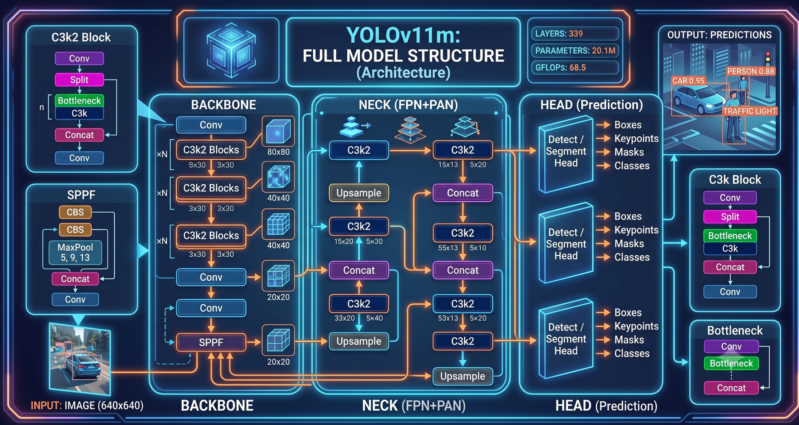
Terminal output showing Ultralytics YOLOv11 model summary: 339 layers, 20.1M parameters, 68.5 GFLOPs, and GPU memory usage during inference — Fig. 1 — `yolo11m.pt` model summary output showing 339 layers, 20.1M parameters, and 68.5 GFLOPs. The model loads in under two seconds on a modern GPU.

Running Inference on Images and Video

The Ultralytics API is intentionally minimal. A single method call handles images, video files, URLs, numpy arrays, and PIL Images. You don’t need to write preprocessing code for basic inference.

Single Image Inference

        python
        infer_image.py
      
from ultralytics import YOLO

model = YOLO(“yolo11m.pt”)  # downloads ~40MB on first run

results = model(“path/to/image.jpg”, conf=0.4, iou=0.45)

for r in results:
    print(f”Detected {len(r.boxes)} objects”)

    # Iterate boxes
    for box in r.boxes:
        cls  = r.names[int(box.cls)]
        conf = float(box.conf)
        x1, y1, x2, y2 = [int(v) for v in box.xyxy[0]]
        print(f”  {cls:15s} conf={conf:.2f}  bbox=[{x1},{y1},{x2},{y2}]”)

    r.save(“result.jpg”)   # writes annotated image
    r.show()               # opens preview window

Live Webcam Inference

        python
        webcam.py
      
from ultralytics import YOLO
import cv2

model = YOLO(“yolo11n.pt”)  # nano for real-time webcam
cap   = cv2.VideoCapture(0)

while cap.isOpened():
    ret, frame = cap.read()
    if not ret:
        break

    # stream=True returns a generator — more memory-efficient for video
    for r in model(frame, stream=True, verbose=False):
        annotated = r.plot()              # draws boxes + labels
        cv2.imshow(“YOLOv11”, annotated)

    if cv2.waitKey(1) & 0xFF == ord(“q”):
        break

cap.release()
cv2.destroyAllWindows()

Pass stream=True for any video source. Without it, Ultralytics accumulates all results in memory before returning — fine for a single image, a bottleneck for a two-hour security recording.

Training on Your Own Data

Pretrained COCO weights cover 80 classes well, but any specialized domain — medical imaging, retail shelf analysis, agricultural defect detection — needs custom training. The process has four stages.

Collect and Annotate Images

500–1,000 labeled images per class is enough to fine-tune meaningfully from COCO weights. Use Roboflow, Label Studio, or CVAT for annotation. Export in YOLO format (one .txt file per image, each line: class cx cy w h in normalized coordinates).

Organize the Dataset Directory

Ultralytics expects a specific folder structure. Images and labels live in parallel directories, split into train/, val/, and optionally test/. A YAML file ties it together.

Write the data.yaml Config

This file tells the trainer where your data lives and what your classes are named. Get this file right before touching any Python code — a misconfigured YAML is the most common first-time training error.

Run Training and Monitor

Call model.train() with your config. Ultralytics saves checkpoints every epoch and automatically runs validation at the end. Check runs/train/ for results, confusion matrices, and PR curves.

Dataset Directory Structure

        text
        folder structure
      
my_dataset/
├── images/
│   ├── train/     # your training images (.jpg / .png)
│   ├── val/       # validation images (~15% of total)
│   └── test/      # held-out test images (optional)
└── labels/
    ├── train/     # one .txt per image, same filename
    ├── val/
    └── test/

data.yaml Config File

        yaml
        data.yaml
      
# Absolute path to your dataset root
path: /home/user/my_dataset

train: images/train
val:   images/val
test:  images/test   # optional

# Number of classes and their names (order matters — must match label files)
nc: 3
names:
  0: car
  1: person
  2: bicycle

Training Script

        python
        train.py
      
from ultralytics import YOLO

# Start from COCO pretrained weights for faster convergence
model = YOLO(“yolo11m.pt”)

results = model.train(
    data=“data.yaml”,
    epochs=100,
    imgsz=640,        # input resolution — 640 is standard
    batch=16,         # reduce to 8 if GPU OOM
    device=“cuda”,    # “cpu” for CPU-only machines
    patience=20,      # early stopping: stop if no improvement for 20 epochs
    lr0=0.01,         # initial learning rate
    lrf=0.01,         # final lr = lr0 * lrf
    weight_decay=0.0005,
    augment=True,     # mosaic, flips, HSV jitter enabled by default
    project=“runs/train”,
    name=“my_detector”,
    exist_ok=True,
)

print(f”Best mAP@50: {results.results_dict[‘metrics/mAP50(B)’]:.4f}”)
print(f”Best weights saved to: {results.save_dir}/weights/best.pt”)

Training 100 epochs on a T4 GPU with a 3,000-image dataset takes roughly 45–75 minutes. Ultralytics saves best.pt (highest validation mAP) and last.pt (final epoch) automatically. Always deploy best.pt, not last.pt.

“The difference between a model that reaches 85% mAP and one that stalls at 60% is almost always in the data, not the architecture. More diverse images, better labels, and correct augmentation configuration outperform any hyperparameter change.”

— Consistent finding across dozens of custom YOLOv11 fine-tuning projects

Validating Your Trained Model

Never trust training loss curves alone. Run a proper validation pass against your held-out test set and read each metric carefully before calling a model production-ready.

        python
        validate.py
      
from ultralytics import YOLO

model = YOLO(“runs/train/my_detector/weights/best.pt”)

metrics = model.val(
    data=“data.yaml”,
    split=“test”,     # use the held-out test split
    conf=0.4,
    iou=0.45,
    verbose=True,
)

print(f”mAP@50:      {metrics.box.map50:.4f}”)
print(f”mAP@50-95:  {metrics.box.map:.4f}”)
print(f”Precision:   {metrics.box.mp:.4f}”)
print(f”Recall:      {metrics.box.mr:.4f}”)

# Per-class breakdown
for i, name in model.names.items():
    print(f”  {name}: mAP50={metrics.box.maps[i]:.4f}”)

What to look for in the metrics:

mAP@50

≥0.80

Mean Average Precision at 50% IoU overlap. The headline metric. Below 0.70 for a production use case usually means more training data is needed.

mAP@50-95

≥0.55

Averaged across IoU thresholds 0.50–0.95. Penalizes loose bounding boxes. Important when precise localization matters (robotics, medical).

Precision

≥0.85

Of all predicted boxes, how many were correct. Low precision means false alarms — the model fires on things that aren’t there.

Recall

≥0.80

Of all real objects, how many were found. Low recall means missed detections — objects that were there but the model didn’t report.

Precision and recall sit in tension: lowering your confidence threshold finds more objects (better recall) but also more false positives (worse precision). Set the threshold for your use case — a security system tolerates false alarms better than a medical device does.

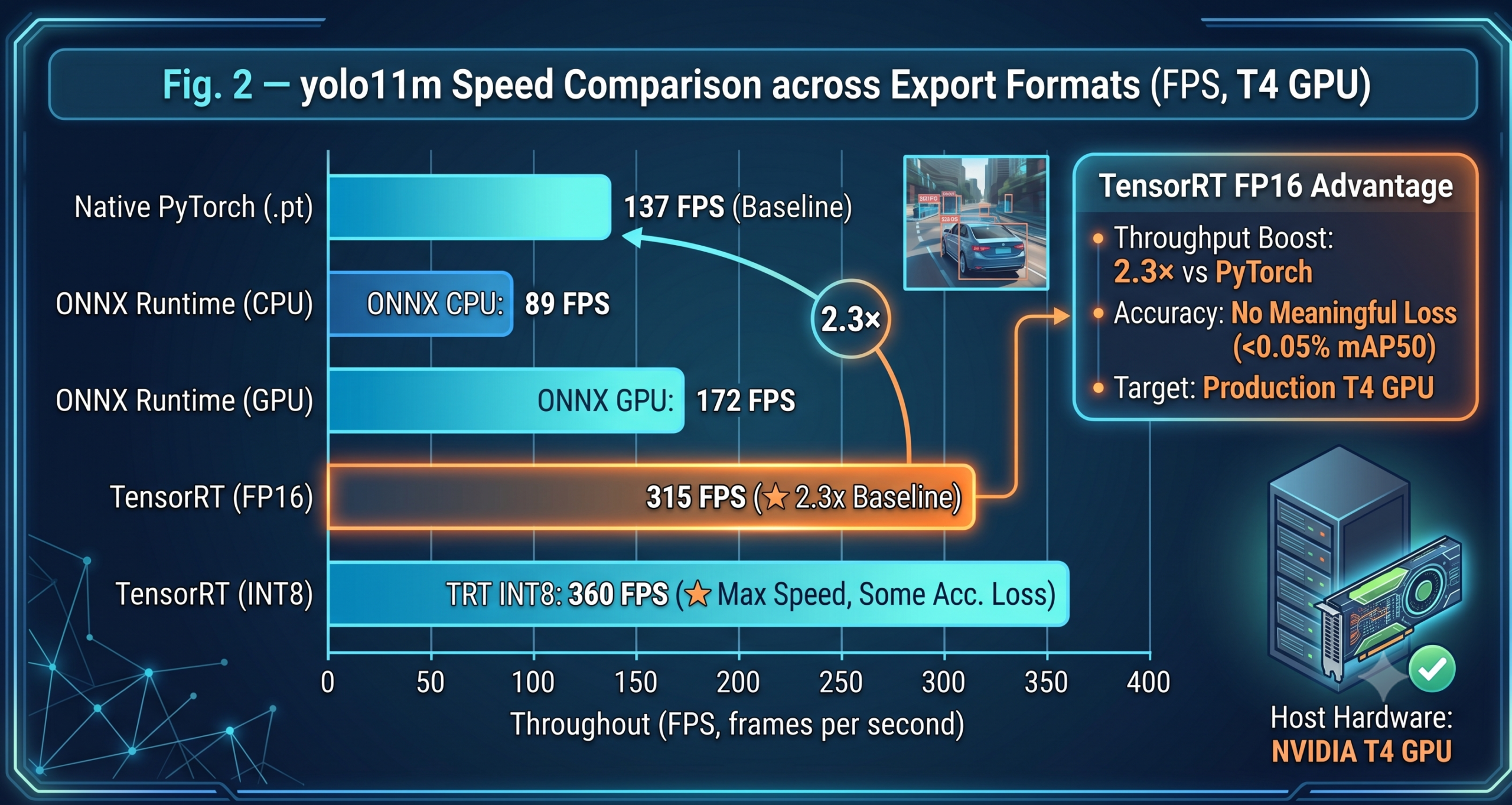
Exporting Your Model for Deployment

The .pt PyTorch weights file requires PyTorch at runtime. For production deployments, export to a format that removes that dependency and runs faster in inference-only mode.

        python
        export.py
      
from ultralytics import YOLO

model = YOLO(“runs/train/my_detector/weights/best.pt”)

# ONNX — runs anywhere: servers, edge, mobile, browsers via onnxruntime
model.export(
    format=“onnx”,
    imgsz=640,
    dynamic=True,     # variable batch size at runtime
    simplify=True,    # graph simplification for smaller file
    opset=17,
)
# Creates: runs/train/my_detector/weights/best.onnx

# TensorRT — NVIDIA GPUs only, highest throughput, FP16 quantization
model.export(
    format=“engine”,
    imgsz=640,
    half=True,     # FP16 halves memory, adds ~10–20% speed
    workspace=4,   # GB of GPU workspace for TRT optimization
)
# Creates: runs/train/my_detector/weights/best.engine

# CoreML — Apple Silicon and iOS deployment
model.export(format=“coreml”, imgsz=640, nms=True)

# TFLite — Android and microcontrollers
model.export(format=“tflite”, imgsz=640, int8=True)

Comparison chart showing inference speed improvements: YOLOv11m in PyTorch at 90 FPS, ONNX at 115 FPS, TensorRT FP16 at 210 FPS on a T4 GPU — Fig. 2 — Speed comparison of yolo11m across export formats on an NVIDIA T4 GPU. TensorRT FP16 delivers 2.3× the throughput of native PyTorch at no accuracy cost under normal conditions.

Deploying a Detection API with FastAPI

For most web and microservice deployments, wrapping your model in a FastAPI endpoint is the fastest path to production. The endpoint accepts an uploaded image file and returns JSON detections.

        python
        api.py
      
import numpy as np
from fastapi import FastAPI, File, UploadFile, Query
from fastapi.responses import JSONResponse
from PIL import Image
from io import BytesIO
from ultralytics import YOLO

app   = FastAPI(title=“YOLOv11 Detection API”, version=“1.0”)
model = YOLO(“best.pt”)  # loaded once at startup, reused per request

@app.get(“/”)
async def health():
    return {“status”: “ok”, “model”: “yolo11m”}

@app.post(“/detect”)
async def detect(
    file: UploadFile = File(…),
    conf: float      = Query(0.4, ge=0.1, le=1.0),
    iou:  float      = Query(0.45, ge=0.1, le=1.0),
):
    img_bytes = await file.read()
    img = Image.open(BytesIO(img_bytes)).convert(“RGB”)
    img_array = np.array(img)

    results = model(img_array, conf=conf, iou=iou, verbose=False)
    detections = []
    for r in results:
        for box in r.boxes:
            detections.append({
                “class”:      r.names[int(box.cls)],
                “confidence”: round(float(box.conf), 4),
                “bbox”:       [int(v) for v in box.xyxy[0].tolist()],
            })

    return JSONResponse({
        “detections”: detections,
        “count”:      len(detections),
        “image_size”: [img.width, img.height],
    })

        bash
        run the server
      
# Start the API server on port 8000
uvicorn api:app –host 0.0.0.0 –port 8000

# Test with curl
curl -X POST http://localhost:8000/detect \
  -F “file=@test_image.jpg” \
  -G –data-urlencode “conf=0.4”

One important production detail: the YOLO("best.pt") call happens at module load time, not inside the endpoint function. This means the model initializes once when the server starts and is reused for every request. If you load the model inside the endpoint, every request pays a 2–5 second initialization penalty — an easy mistake that kills throughput.

Deployment Options by Use Case

REST API

FastAPI + Uvicorn

The setup above. Containerize with Docker and deploy to any cloud. Best for 10–500 requests per second with a GPU-backed server.

Edge

ONNX Runtime

Export to ONNX and run via onnxruntime on Raspberry Pi, Jetson Nano, or industrial PLCs without a GPU. The nano model hits real-time on a Jetson Orin.

Cloud GPU

TensorRT Engine

Export to TensorRT for NVIDIA server GPUs. FP16 mode doubles throughput over ONNX at no meaningful accuracy loss. Requires CUDA-capable hardware at inference time.

Mobile

CoreML / TFLite

CoreML for iOS and Apple Silicon. TFLite with INT8 quantization for Android. The nano model runs at 25–40 FPS on a mid-range smartphone after quantization.

YOLOv11 vs Previous Versions

If you’re migrating from an older YOLO version, here’s where YOLOv11 stands relative to its predecessors and a transformer-based competitor:

Model	mAP@50-95 (COCO)	Params	FPS (T4 GPU)	Best Fit
YOLOv5n	28.0	1.9M	~230	Legacy edge systems
YOLOv8n	37.3	3.2M	~180	Previous edge standard
YOLOv11n	39.5	2.6M	~190	Current edge standard
YOLOv8s	44.9	11.2M	~130	Balanced (older)
YOLOv11s	47.0	9.4M	~140	Balanced (current)
YOLOv11m	51.5	20.1M	~90	Production default
YOLOv11l	53.4	25.3M	~65	High-accuracy server
YOLOv11x	54.7	56.9M	~35	Maximum accuracy
RT-DETR-L	53.0	32.0M	~55	Transformer alternative

The pattern is consistent: every YOLOv11 variant achieves higher mAP than its YOLOv8 counterpart while using fewer parameters. If you’re running YOLOv8 in production today, switching to the equivalent YOLOv11 size is a free accuracy upgrade with no infrastructure change required.

Common Training Problems and Fixes

Three issues trip up most first-time YOLOv11 users:

mAP plateaus early and stops improving: Check your val split for label noise first. A contaminated validation set makes the model look like it stopped learning when it’s actually still improving against your test set. Also try reducing lr0 to 0.001 for small datasets under 1,000 images.
CUDA out of memory during training: Halve your batch size before reducing image size. Batch 8 at 640px trains better than batch 16 at 416px. If you’re still OOM, add half=True to enable FP16 training.
Lots of false positives at low confidence: Your negative examples (images with no labeled objects) may be missing from the dataset. YOLO learns from what’s absent as much as what’s present. Include dedicated background images — roughly one negative for every four positive images is a reasonable ratio.

Before You Deploy

Run your best.pt model on at least 50 images from production conditions — not from your curated test split. Real deployment images often have different lighting, compression artifacts, partial occlusions, or aspect ratios that your training data didn’t cover. Catching distribution shift before deployment is an afternoon of work. Catching it after a week of bad predictions in production is considerably more painful.

What YOLOv11 Cannot Do

No model is universal. YOLOv11 struggles in three specific scenarios you should know before committing to it for your use case.

Dense small-object scenes — satellite imagery with hundreds of tiny vehicles, microscopy slides with thousands of cells — require specialized approaches. YOLOv11 was designed for objects that occupy at least 1–2% of the image area. Below that, you need tiling strategies or specialized architectures like SAHI (Slicing Aided Hyper Inference).

Class imbalance above 50:1 is problematic. If you have 10,000 images of class A and 200 of class B, the model will confidently detect A and poorly detect B regardless of what hyperparameters you set. Solve this with data — collect more examples of minority classes or use augmentation pipelines that oversample them.

Finally, YOLO is a detection model, not a recognition model. It tells you there’s a car; it cannot tell you which specific car it is. For identity tasks (face recognition, vehicle re-identification, product SKU lookup), you need a separate embedding or classification head on top of the detector’s output.

Build the Full Pipeline Around Your Detector

YOLOv11 is one component. See how to connect it to OCR, batch processors, and production APIs in our Computer Vision Pipelines guide — built with Claude Code.

CV Pipelines with Claude Code Try Claude AI

Share on Facebook

Post on X

Save