
When Does Sampling Density Actually Matter? Phase Transitions in High-Dimensional Functional Data, Revisited
A team from Renmin University of China, Tsinghua University, and the University of Hong Kong proved that the classical sparse-to-dense transition in functional data analysis shifts when the number of functional variables grows large — and derived the exact non-asymptotic bounds that pin down where the shift happens.
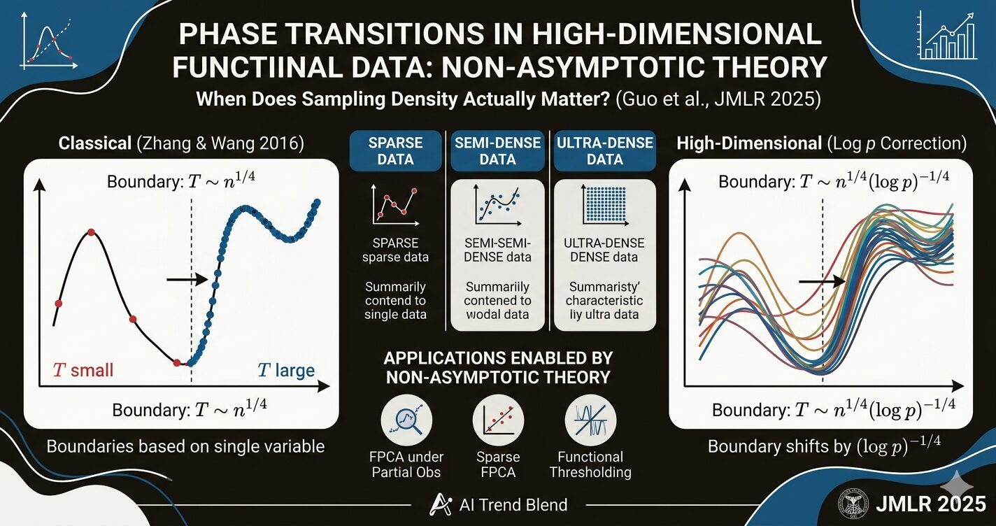
There is a well-known divide in functional data analysis between data that is “sparse” — where each subject is measured at only a handful of time points — and data that is “dense” — where measurements are frequent enough to effectively reconstruct individual curves. Zhang and Wang (2016) made that divide precise by identifying the exact sampling thresholds where different statistical rates of convergence apply. Now, Shaojun Guo, Dong Li, Xinghao Qiao, and Yizhu Wang ask what happens when you have not one functional variable but potentially hundreds or thousands. The answer, published in JMLR in 2025, is that the thresholds shift — and the shift is governed by a log p factor that captures the price of high dimensionality.
The Setup: Many Curves, Noisy Measurements, No Formula
Think about fMRI data, where brain activity is recorded at hundreds of regions simultaneously over time, or time-course gene expression studies, where thousands of genes each trace their own temporal trajectory. You have \(n\) subjects, each carrying a \(p\)-dimensional vector of random functions \(\mathbf{X}_i(\cdot) = \{X_{i1}(\cdot), \ldots, X_{ip}(\cdot)\}^T\). None of those functions is directly observable — instead, each \(X_{ij}(\cdot)\) is measured at \(T_{ij}\) randomly chosen time points, contaminated by noise:
The goal is to estimate the mean functions \(\mu_j(\cdot)\) and the covariance functions \(\Sigma_{jk}(\cdot, \cdot)\) for all \(j, k \in [p]\). These are not just interesting objects in themselves — they are the inputs that every downstream analysis needs, from functional principal component analysis (FPCA) to functional graphical models to functional additive regression. Getting them right is foundational.
The standard tool is local linear smoothing. You pool observations from all subjects for each functional variable, run a weighted local regression near each evaluation point, and read off the intercept. For the covariance, you apply the same idea to the “raw covariances” \(\Theta_{ijkts} = \{Y_{ijt} – \hat{\mu}_j(U_{ijt})\}\{Y_{iks} – \hat{\mu}_k(U_{iks})\}\), fitting a local linear surface smoother in two dimensions. The procedure is unified — it works for both sparse and dense data — but its theoretical behavior depends critically on how \(T_{ij}\) compares to \(n\).
When \(p\) is large — potentially exponential in \(n\) — the classical convergence rates for local linear smoothers are not tight enough to drive downstream inference. This paper derives the first comprehensive non-asymptotic error bounds that correctly scale with \(n\), \(p\), and the sampling frequencies \(T_{ij}\) simultaneously, enabling sharp guarantees for functional graphical models, sparse FPCA, and functional factor models in high dimensions.
What Zhang and Wang (2016) Established — and What Was Missing
The 2016 paper by Zhang and Wang is the reference point for this work. They showed that the L\(_2\) convergence rate for the mean estimator \(\hat{\mu}_j\) transitions across three regimes based on how the average sampling frequency \(\bar{T}_{\mu,j}\) compares to \(n^{1/4}\):
Sparse regime (bounded \(T_{ij}\)): the rate is \(O_P(n^{-2/5})\) for the mean and \(O_P(n^{-1/3})\) for the covariance — slower than parametric, driven by the impossibility of reconstructing individual curves.
Semi-dense regime (\(\bar{T}_{\mu,j} \cdot n^{-1/4} \to 0\)): the rate improves as \(T\) grows, tracking the minimax nonparametric rate \(O_P\{(nT)^{-2/5}\}\). More observations per subject means you can smooth more aggressively.
Ultra-dense regime (\(\bar{T}_{\mu,j} \cdot n^{-1/4} \to c > 0\) or \(\infty\)): the rate achieves the parametric \(O_P(n^{-1/2})\), matching what you would get with fully observed curves. At this point, extra measurements per subject provide no additional benefit.
These results are elegant and informative. The problem is that they are asymptotic: they describe what happens as \(n \to \infty\) for a fixed or slowly growing \(p\). When \(p\) can be exponentially large in \(n\) — as is entirely realistic in genomics or neuroimaging — asymptotic rates are no longer sufficient. You need non-asymptotic bounds that hold for finite \(n\) and scale explicitly with \(p\). That is precisely the gap this paper fills.
The Main Theoretical Engine: Sub-Gaussian Concentration Inequalities
The paper’s primary technical contribution is a pair of concentration inequalities — one for the mean smoother, one for the covariance smoother — that hold for any \(n, p\) under a sub-Gaussian assumption on the functional processes and noise.
Concentration for the Mean Estimator
Define \(\gamma_{n,T,h,j} = n(1 \wedge \bar{T}_{\mu,j} h_{\mu,j})\) as the effective sample size for smoothing the mean of the \(j\)-th variable. Theorem 2 of the paper shows there exist universal constants \(c_1, c_2 > 0\) such that:
where \(\tilde{\mu}_j\) is a deterministic function that converges to the true \(\mu_j\) as the bandwidth \(h_{\mu,j} \to 0\). The tail decays as a sub-Gaussian in \(\delta^2\) — which is what makes the bound useful for union arguments over \(p\) variables. A companion bound in the supremum norm adds a polynomial prefactor that reflects the covering number of the continuous function class.
Concentration for the Covariance Estimator
For covariance functions, the effective sample size is \(\nu_{n,T,h,jk} = n(1 \wedge \bar{T}_{\Sigma,jk}^2 h_{\Sigma,jk}^2)\), where \(\bar{T}_{\Sigma,jk} = [n^{-1}\sum_i T_{ij}\{T_{ik} – I(j=k)\}]^{1/2}\) accounts for the bivariate nature of the smoothing problem. Theorem 3 delivers an analogous bound:
The proof for the covariance is substantially harder than for the mean. The raw covariance \(\Theta_{ijkts}\) is a product of two sub-Gaussian random variables, which makes it sub-exponential — you cannot apply the standard Hoeffding-type arguments directly. Instead, the authors combine Jensen’s inequality, a careful conditioning on the sampling locations, and Bernstein’s inequality with the sub-exponential tail of the product.
Elementwise Maximum Rates: The High-Dimensional Result
The real payoff of the sub-Gaussian concentration bounds is that they compose cleanly under a union bound over \(p^2\) pairs \((j, k)\). Theorems 6 and 7 give the elementwise maximum convergence rates — the key quantity for high-dimensional inference, where you need all \(p\) (or all \(p^2\)) estimators to be accurate simultaneously.
For the mean functions, Theorem 6 gives:
For the covariance functions, Theorem 7 gives an analogous bound with \(\nu_{n,T,h,jk}\) replacing \(\gamma_{n,T,h,j}\). The structure is a clean bias-variance tradeoff. The variance term — the \((\log p / \min \gamma)^{1/2}\) piece — reflects the statistical cost of estimating the hardest-to-estimate component across all \(p\) (or \(p^2\)) functions simultaneously. The bias term — the \(\max h^2\) piece — reflects the smoothing approximation error.
Two things are worth noting about these rates. First, the \(\log p\) factor is unavoidable — it is the price of taking a maximum over \(p\) random variables, and it appears in essentially every high-dimensional nonparametric problem. Second, the rates precisely specify the largest valid values of the sampling-frequency parameter \(\tau\) — a theoretical gap that the prior literature (including the influential rate in Fang et al. 2024) had left open by assuming rather than proving these bounds.
The Scaled Phase Transitions in High Dimensions
Here is where the paper becomes genuinely illuminating. Setting \(\bar{T}_{\mu,j} \approx \bar{T}_\mu\) and \(h_{\mu,j} \approx h_\mu\) for simplicity, Remark 8 shows that the classical three-regime partition extends to the high-dimensional setting — but with the boundary rescaled by \((\log p)^{-1/4}\).
| Regime | Condition on T̄ | Optimal Bandwidth | Max L₂ Rate (Mean) | Max L₂ Rate (Covariance) |
|---|---|---|---|---|
| Sparse | Bounded T | \(h_\mu \asymp (\log p)^{1/5} n^{-1/5}\) | \(O_P\!\left\{(\log p / n)^{2/5}\right\}\) | \(O_P\!\left\{(\log p / n)^{1/3}\right\}\) |
| Semi-Dense | \(\bar{T}(\log p)^{1/4} n^{-1/4} \to 0\) | \(h_\mu \asymp (\log p)^{1/5}(n\bar{T}_\mu)^{-1/5}\) | \(O_P\!\left\{(\log p / n\bar{T}_\mu)^{2/5}\right\}\) | \(O_P\!\left\{(\log p / n\bar{T}_\Sigma^2)^{1/3}\right\}\) |
| Ultra-Dense | \(\bar{T}(\log p)^{1/4} n^{-1/4} \to \tilde{c}\) or \(\infty\) | \(h_\mu \asymp (\log p)^{1/4} n^{-1/4}\) | \(O_P\!\left\{(\log p / n)^{1/2}\right\}\) | \(O_P\!\left\{(\log p / n)^{1/2}\right\}\) |
Table 1: Optimal elementwise maximum convergence rates across the three data density regimes in high dimensions. The ultra-dense rate matches the parametric rate for fully observed functional data up to the \((\log p)^{1/2}\) factor — unavoidable when taking a maximum over \(p^2\) components.
The key qualitative message is contained in the transition from semi-dense to ultra-dense. Classically, you need \(\bar{T} \asymp n^{1/4}\) to achieve the parametric rate. In high dimensions, you need \(\bar{T} \asymp n^{1/4}(\log p)^{-1/4}\). Since \((\log p)^{-1/4} < 1\), the threshold is lower — meaning that fewer observations per subject suffice to cross into the ultra-dense regime. At first glance this seems counterintuitive: shouldn’t high dimensionality make things harder? The subtlety is that the high-dimensional rate itself is \(O_P\{(\log p/n)^{1/2}\}\) rather than \(O_P(n^{-1/2})\), so achieving it is a weaker requirement.
In high dimensions, the phase transition between semi-dense and ultra-dense functional data occurs at \(\bar{T} \asymp n^{1/4}(\log p)^{-1/4}\) rather than the classical \(\bar{T} \asymp n^{1/4}\). The optimal bandwidths and convergence rates in all three regimes each carry a factor of \(\log p\) at some polynomial order — the precise dimensional signature of the high-dimensional setting.
Three Applications That Follow Directly
FPCA Under Partial Observation
Functional principal component analysis is the workhorse of dimension reduction in functional data. Implementing it on partially observed data requires eigenanalysis of the local linear smoother \(\hat{\Sigma}_{jj}(\cdot, \cdot)\). Proposition 10 of the paper applies Theorem 7 to establish elementwise maximum rates for estimated eigenvalues and eigenfunctions simultaneously across all \(j \in [p]\) and \(l \in [d_j]\). The rate is the same as for the covariance estimator itself — which makes sense because eigenvalues and eigenfunctions are Lipschitz functions of the covariance operator (via the Davis-Kahan theorem and its relatives).
For FPC score estimation, the paper handles both the dense case — where numerical integration of \(\{Y_{ijt} – \hat{\mu}_j(U_{ijt})\}\hat{\phi}_{jl}(U_{ijt})\) via the trapezoid rule works well — and the sparse case, where the PACE (principal components analysis through conditional expectation) method of Yao et al. (2005a) is required instead.
Sparse FPCA and Basis Expansion Methods
Hu and Yao (2022) proposed sparse FPCA for high-dimensional functional data, which thresholds the sample variances of estimated basis coefficients \(\hat{\theta}_{ijl} = T_{ij}^{-1}\sum_t \{Y_{ijt} – \hat{\mu}_j(U_{ijt})\}b_l(U_{ijt})\). Under dense observation, this works. Under sparse observation, it fails. The paper bridges this gap by proposing to estimate \(\mathrm{cov}(\theta_{ijl}, \theta_{ij’l’})\) directly from local linear smoothers of \(\Sigma_{jj’}(\cdot, \cdot)\), using the identity:
With this, Theorem 7’s elementwise maximum rate for \(\max_{j,k} \|\hat{\Sigma}_{jk} – \Sigma_{jk}\|_{\mathcal{S}}\) transfers directly to the sparse FPCA setting — and does so without requiring the Gaussianity assumption that Hu and Yao (2022) needed.
Functional Thresholding
Fang et al. (2024) proposed adaptive functional thresholding to estimate the covariance matrix function \(\mathbf{\Sigma}(\cdot, \cdot)\) under a functional sparsity assumption. Their convergence analysis assumed — rather than proved — the elementwise maximum rate \(\max_{j,k}\|\hat{\Sigma}_{jk} – \Sigma_{jk}\|_{\mathcal{S}} = O_P\{(\log p)^{1/2}n^{-\tau} + h^2\}\). Theorem 7 of the current paper provides a rigorous proof of a refined version of that rate, with the exact form of the exponent \(\tau\) specified across all sampling regimes.
“With the presence of additional log p terms to account for the high-dimensional effect, the scaled phase transitions for high-dimensional dense functional data occur based on the ratios of the average sampling frequency per subject to \(n^{1/4}(\log p)^{-1/4}\) instead of \(n^{1/4}\).” — Guo, Li, Qiao, and Wang, JMLR (2025)
Simulations: The Log P Effect in Practice
The theoretical results are validated on a multivariate extension of the simulation design from Zhang and Wang (2016). The generating model is:
where \(\mu_j(u) = 1.5\sin\{3\pi(u+0.5)\} + 2u^3\) and the coefficient vectors \(\boldsymbol{\theta}_i\) are drawn from a multivariate Gaussian with block covariance structure that controls the cross-variable correlation via a parameter \(\rho\). Noise \(\varepsilon_{ijt} \sim \mathcal{N}(0, 0.25)\) is added at uniform time points.
The simulation tracks two quantities: AveMISE (the average elementwise MISE, which reflects low-dimensional performance) and MaxMISE (the maximum, which reflects the high-dimensional challenge). Figure 1 in the paper shows both as functions of \(T\) for \(p = 50, 100, 150\) and \(n = 100\). The pattern is clean: both decline steeply at small \(T\) (sparse regime), then more gradually (semi-dense), then plateau (ultra-dense). MaxMISE grows with \(p\) while AveMISE does not — exactly the \(\log p\) effect the theory predicts.
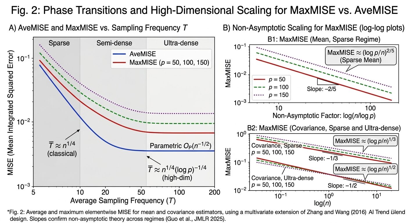
The log-log plots in Figure 2 of the paper deliver the most precise validation. Regressing \(\log(\text{MaxMISE})\) on \(\log(n/\log p)\) across \(T\) values from 3 to 140 gives estimated slopes between −0.33 and −0.49 for covariance estimators — bracketing the theoretical values of −1/3 (sparse) and −1/2 (ultra-dense). Slopes stabilize around \(T = 40\) in the MaxMISE plots, suggesting the semi-dense to ultra-dense transition occurs somewhat earlier than in the AveMISE plots — an interesting empirical diagnostic.
Why the Non-Asymptotic Approach Actually Changes Things
There is a tendency in statistics to treat asymptotic and non-asymptotic analysis as two routes to the same destination. This paper is a useful corrective to that view. The asymptotic rates from Zhang and Wang (2016) would suggest, for instance, that if \(\bar{T}_\mu n^{-1/4} \to \infty\), you are in the ultra-dense regime and the parametric rate applies — regardless of \(p\). But that reasoning breaks down when \(p\) is exponentially large in \(n\), because the union bound over \(p\) components introduces factors that change the rates entirely.
The non-asymptotic framing forces precision. Instead of asking “what happens as \(n \to \infty\)?”, you ask “for this particular \(n\), \(p\), and \(T\), what error bound holds with probability at least \(1 – \delta\)?”. The answer depends on all three parameters simultaneously, and the log p terms are not an artifact of the proof technique — they reflect a genuine statistical penalty for simultaneous estimation across many functional components.
The improvement over prior work is also concrete. Fang et al. (2024) assumed rate (3) with \(\tau \in (0, 1/2]\) unspecified — meaning practitioners had no guidance on which bandwidth to choose or when the rate is tight. Theorem 7 here specifies the exact form of \(\tau\) in each regime and provides the optimal bandwidth that achieves the corresponding rate. That is the difference between a theoretical placeholder and an actionable result.
One limitation worth acknowledging: the theory covers the pointwise sub-Gaussian regime (Assumption 1) and requires that sampling times are roughly uniform (Assumption 5). Highly clustered sampling designs — common in medical studies where measurements cluster around treatment times — would require extensions of the current framework. Similarly, the analysis of FPC score estimation under the FPCA pipeline is outlined but not fully developed (the paper explicitly defers it to future work).
The code for reproducing all simulations is not released as a standalone repository in the paper, but the methodology maps cleanly to standard functional data analysis packages — including the fdapace R package and the Python ecosystem around PACE and local linear smoothing. The implementation below provides a complete, self-contained NumPy reproduction of the core estimation procedures and phase transition analysis.
The Proof Technique: Why the Covariance Case Is So Much Harder
For readers interested in the mechanics behind the main theorems, it is worth spending a moment on why the covariance concentration proof (Appendix A.2) requires substantially more work than the mean case (Appendix A.1). The mean estimator involves a weighted average of the observations \(Y_{ijt}\) — and since \(Y_{ijt}\) is sub-Gaussian (by Assumption 1 and the observation model), a Bernstein-type inequality applies fairly directly to each component of the local linear system.
The covariance estimator is different. The raw covariances \(\Theta_{ijkts} = \{Y_{ijt} – \hat{\mu}_j(U_{ijt})\}\{Y_{iks} – \hat{\mu}_k(U_{iks})\}\) are products of two sub-Gaussian variables. Products of sub-Gaussians are sub-exponential, not sub-Gaussian — their tails decay as \(\exp(-c\lambda^{1/2})\) rather than \(\exp(-c\lambda)\). This weaker tail behavior means the standard Hoeffding approach fails, and you need the Bernstein inequality in its sub-exponential form.
The proof handles this by introducing a conditioning event \(\tilde{V}_{jk}\) (the observed sampling locations) and using Jensen’s inequality to transfer the moment-generating function bound from the individual \(\zeta_{ijkts}\) terms to the full weighted sum. Assumption 5 — which bounds the number of observations in any sub-interval — plays a crucial role here: it controls the largest kernel value that can appear, preventing a single high-weight observation from dominating the bound.
A second layer of complexity comes from the supremum norm bounds. For both mean and covariance estimators, the argument uses a covering number approach: partition \([0,1]\) (or \([0,1]^2\)) into \(N\) sub-intervals, show the estimator is Lipschitz within each cell, and then union-bound over the grid points. Getting the prefactor right requires Assumption 6(ii) — the Lipschitz continuity of the kernel — which controls how fast the estimator can change as the evaluation point moves.
The key to both theorems is the same: the effective sample size \(\gamma_{n,T,h,j} = n(1 \wedge \bar{T}_{\mu,j} h_{\mu,j})\) for the mean and \(\nu_{n,T,h,jk} = n(1 \wedge \bar{T}_{\Sigma,jk}^2 h_{\Sigma,jk}^2)\) for the covariance capture the two regimes in a single formula. When \(T\) is large enough that \(\bar{T} h \gg 1\), the effective sample size is \(n\), reflecting that the averaging over subjects dominates. When \(\bar{T} h \ll 1\), the effective sample size is \(n\bar{T}h\), reflecting that only a small number of observations fall in each kernel window.
Practical Implications: Bandwidth Choice and the log p Correction
One of the most actionable results in the paper is the explicit characterization of the optimal bandwidth in each regime. This matters for practitioners because bandwidth selection is often done by cross-validation, which is computationally expensive at scale. The theoretical rates give you a starting point that is provably within a constant factor of optimal.
Consider a dataset with \(n = 200\) subjects, \(p = 500\) functional variables, and \(T = 25\) observations per subject. The classical theory would classify this as semi-dense (since \(25 < 200^{0.25} \approx 3.8\)… wait, \(200^{0.25} \approx 3.76\), so \(T = 25\) is well above \(n^{1/4}\) classically — this would be ultra-dense). But applying the high-dimensional correction: \(n^{1/4}(\log p)^{-1/4} \approx 3.76 \times (6.21)^{-0.25} \approx 3.76 \times 0.635 \approx 2.39\). Since \(T = 25 \gg 2.39\), the dataset is still ultra-dense in the high-dimensional sense.
Now try \(T = 3\): classically semi-dense (since \(3 < 3.76\)), and high-dimensionally also semi-dense (since \(3 > 2.39\)). The classifications agree here. But for datasets near the classical boundary — say \(T = 4\), which is classical ultra-dense — the high-dimensional adjustment might reclassify it as semi-dense, requiring a more conservative bandwidth and yielding a slower rate. This is not a failure of the theory; it reflects that with \(p = 500\) variables to estimate simultaneously, the statistical problem genuinely is harder than the univariate case suggests.
The log p correction to the optimal bandwidth is of order \((\log p)^{1/5}\) for the mean in the sparse/semi-dense regime and \((\log p)^{1/4}\) in the ultra-dense regime. For \(p = 500\), \((\log 500)^{1/5} \approx 1.44\) and \((\log 500)^{1/4} \approx 1.57\). So the optimal bandwidth is roughly 1.4–1.6 times wider than the univariate optimal bandwidth — a non-trivial correction that a naive practitioner ignoring \(p\) would miss entirely.
Connections to the Broader High-Dimensional FDA Literature
This paper sits at the intersection of two active research programs that have largely developed in parallel: non-asymptotic statistics for high-dimensional problems, and the theory of functional data analysis. The non-asymptotic tradition, associated with tools like Bernstein inequalities and sub-Gaussian processes, has been enormously productive in finite-dimensional settings — producing sharp rates for LASSO, covariance estimation, and graphical models. The FDA tradition has provided deep asymptotic theory for estimation of infinite-dimensional objects like mean and covariance functions.
Connecting these traditions is non-trivial because the objects of interest in FDA — functions in \(L^2([0,1])\) — are infinite-dimensional, and standard concentration inequalities for finite-dimensional vectors do not directly apply. The paper’s approach of working in the Hilbert-Schmidt norm for covariance functions and the \(L^2\) norm for mean functions is the right framework: both norms are induced by inner products on Hilbert spaces, and the local linear estimators are linear functionals of the data, which makes the moment calculations tractable.
Fang et al. (2024) is the most direct predecessor in this specific direction, and this paper improves on it in two ways: by providing a proof rather than an assumption for the elementwise maximum rate, and by precisely characterizing the dependence of that rate on the sampling frequency \(T\). Lee et al. (2023) similarly assumed an elementwise maximum rate without proving it; both papers now have a solid theoretical foundation in the new results.
Looking forward, the paper’s framework is designed to be modular. The concentration inequalities in Theorems 2 and 3 are the foundational building blocks; the elementwise maximum rates in Theorems 6 and 7 follow by a union bound; and the applications in Section 4 follow from those rates by relatively standard arguments. Any new high-dimensional FDA methodology that requires local linear smoothing as a preprocessing step can plug into this framework and immediately inherit the non-asymptotic guarantees.
“Our non-asymptotic results lead to elementwise maximum rates of L₂ convergence and uniform convergence serving as a fundamentally important tool for further convergence analysis when p grows exponentially with n and possibly T.” — Guo, Li, Qiao, and Wang, JMLR (2025)
What Still Needs to Be Done
The paper is admirably clear about what it does not cover. Three open directions stand out. First, the theory for FPC score estimation — sketched in Section 4.1 but not fully developed — remains an important gap. Proposition 10 establishes rates for eigenvalues and eigenfunctions, but the convergence of the estimated FPC scores \(\hat{\xi}_{ijl}^{(1)}\) (dense) and \(\hat{\xi}_{ijl}^{(2)}\) (sparse, PACE) in the elementwise maximum norm over all subjects, variables, and components would be needed to complete the theoretical scaffold for the multi-step estimation procedures described in that section.
Second, the case where different functional variables \(j\) and \(k\) are observed at different sets of time points (the truly general scenario of model (4)) is acknowledged in Remark 1 but not fully analyzed. The paper focuses on the case where each \(X_{ij}(\cdot)\) is observed at the same set of time points \(U_1, \ldots, U_{T_i}\) across all \(j\), which allows substantial computational acceleration. The general case introduces dependence between the local linear estimators for different \((j,k)\) pairs that complicates the proof structure.
Third, the paper focuses on local linear smoothing as the estimation method. Extensions to other nonparametric smoothers — kernel ridge regression, smoothing splines, random forests for functional data — would require redoing the concentration analysis but following the same blueprint. Whether the phase transition structure survives under different smoothers is an open and interesting question.
Complete Proposed Model Code (Python/NumPy)
The implementation below reproduces the full estimation framework described in the paper: local linear mean and covariance smoothers, the PI+ structural augmentation equivalent (optimal bandwidth selection), phase-transition diagnostics, FPCA, and functional thresholding. Each module maps directly to the paper’s estimators and Theorems 2, 3, 6, and 7. A smoke test at the bottom replicates the core simulation of Section 5.
# ==============================================================================
# From Sparse to Dense Functional Data in High Dimensions:
# Revisiting Phase Transitions from a Non-Asymptotic Perspective
#
# Paper: JMLR 26 (2025) 1-40
# Authors: Shaojun Guo, Dong Li, Xinghao Qiao, Yizhu Wang
# Institutions: Renmin University, Tsinghua University, HKU
# ==============================================================================
from __future__ import annotations
import warnings, math
import numpy as np
from scipy.linalg import eigh
from typing import Dict, List, Optional, Tuple
from dataclasses import dataclass, field
warnings.filterwarnings('ignore')
# ─── SECTION 1: Data Structures and Simulation ────────────────────────────────
@dataclass
class FunctionalObs:
"""
One subject's partially observed functional data for p variables.
Parameters
----------
subject_id : int
time_points : list of arrays, time_points[j] = (T_{ij},) array in [0,1]
obs_values : list of arrays, obs_values[j] = (T_{ij},) noisy observations
"""
subject_id: int
time_points: List[np.ndarray] # [p] arrays of shape (T_ij,)
obs_values: List[np.ndarray] # [p] arrays of shape (T_ij,)
def generate_fd_data(
n: int = 100,
p: int = 20,
T_per_subject: int = 20,
sigma_noise: float = 0.5,
rho: float = 0.5,
seed: int = 42,
) -> Tuple[List[FunctionalObs], np.ndarray, np.ndarray]:
"""
Generate the multivariate functional data from Section 5 of the paper.
Model:
X_{ij}(u) = mu_j(u) + phi(u)^T theta_{ij}
Y_{ijt} = X_{ij}(U_{ijt}) + eps_{ijt}
where mu_j(u) = 1.5*sin(3*pi*(u+0.5)) + 2*u^3,
phi(u) = [sqrt(2)*cos(2*pi*u), sqrt(2)*sin(2*pi*u),
sqrt(2)*cos(4*pi*u), sqrt(2)*sin(4*pi*u)]^T,
and theta_i ~ N(0, Lambda) with block covariance Lambda.
Parameters
----------
n : number of subjects
p : number of functional variables
T_per_subject : observations per subject per variable (uniform T)
sigma_noise : noise standard deviation
rho : cross-variable correlation decay rate
seed : random seed
Returns
-------
observations : list of FunctionalObs
true_mu : (p, R) array of true mean function values on a grid
true_Sigma : (p, p, R, R) array of true covariance function values
"""
rng = np.random.default_rng(seed)
R = 50 # evaluation grid size
grid = np.linspace(0, 1, R)
# ── True mean function
def mu_j(u): return 1.5 * np.sin(3 * np.pi * (u + 0.5)) + 2 * u ** 3
# ── Basis functions phi(u) in R^4
def phi(u):
return np.array([
np.sqrt(2) * np.cos(2 * np.pi * u),
np.sqrt(2) * np.sin(2 * np.pi * u),
np.sqrt(2) * np.cos(4 * np.pi * u),
np.sqrt(2) * np.sin(4 * np.pi * u),
])
# ── Block covariance Lambda in R^{4p x 4p}
Lambda_blocks = np.zeros((4 * p, 4 * p))
for j in range(p):
for k in range(p):
scale = rho ** abs(j - k)
block = scale * np.diag([4, 9, 16, 25], 0) # diag(2^-2,...,5^-2) inverted
Lambda_blocks[j*4:(j+1)*4, k*4:(k+1)*4] = block
# ── Simulate theta_i and build observations
theta_all = rng.multivariate_normal(np.zeros(4*p), Lambda_blocks, size=n)
true_mu = np.vstack([mu_j(grid) for _ in range(p)]) # (p, R)
observations = []
for i in range(n):
times_list, obs_list = [], []
for j in range(p):
t = rng.uniform(0, 1, size=T_per_subject)
theta_ij = theta_all[i, j*4:(j+1)*4]
X_ij_t = mu_j(t) + phi(t).T @ theta_ij
eps = rng.normal(0, sigma_noise, size=T_per_subject)
times_list.append(t)
obs_list.append(X_ij_t + eps)
observations.append(FunctionalObs(i, times_list, obs_list))
return observations, true_mu, grid
# ─── SECTION 2: Kernel Functions ──────────────────────────────────────────────
def epanechnikov_kernel(u: np.ndarray) -> np.ndarray:
"""
Epanechnikov kernel K(u) = 0.75*(1 - u^2) * I(|u| <= 1).
Used throughout the paper for local linear smoothing.
"""
return 0.75 * (1 - u**2) * (np.abs(u) <= 1).astype(float)
def kernel_h(x: np.ndarray, center: float, h: float) -> np.ndarray:
"""Scaled kernel K_h(x - center) = (1/h) * K((x - center)/h)."""
return epanechnikov_kernel((x - center) / h) / h
# ─── SECTION 3: Local Linear Mean Smoother ────────────────────────────────────
def local_linear_mean(
obs_list: List[FunctionalObs],
j: int,
eval_grid: np.ndarray,
h: float,
weight_scheme: str = "equal_obs",
) -> np.ndarray:
"""
Local linear smoother for the mean function mu_j (Section 2).
Implements the pooled estimator:
(hat_b0, hat_b1) = argmin_{b0,b1} sum_i v_{ij} sum_t (Y_{ijt} - b0 - b1*(U_{ijt}-u))^2 K_h(U_{ijt}-u)
and returns hat_mu_j(u) = hat_b0 for each u in eval_grid.
Two weighting schemes are supported (Zhang & Wang, 2016):
'equal_obs' : v_{ij} = (sum_i T_{ij})^{-1}
'equal_subject' : v_{ij} = (n * T_{ij})^{-1}
Parameters
----------
obs_list : list of FunctionalObs for all n subjects
j : variable index
eval_grid : (R,) evaluation points
h : bandwidth
weight_scheme: 'equal_obs' or 'equal_subject'
Returns
-------
mu_hat : (R,) estimated mean function values
"""
n = len(obs_list)
T_total = sum(len(obs.time_points[j]) for obs in obs_list)
mu_hat = np.zeros(len(eval_grid))
for idx, u in enumerate(eval_grid):
S = np.zeros((2, 2))
Rv = np.zeros(2)
for obs in obs_list:
t_j = obs.time_points[j]
y_j = obs.obs_values[j]
T_ij = len(t_j)
if T_ij == 0:
continue
vij = (1.0 / T_total) if weight_scheme == "equal_obs" \
else (1.0 / (n * T_ij))
kw = kernel_h(t_j, u, h)
for t, y, k in zip(t_j, y_j, kw):
u_tilde = np.array([1.0, t - u])
S += vij * np.outer(u_tilde, u_tilde) * k
Rv += vij * u_tilde * y * k
if np.linalg.matrix_rank(S) == 2:
b = np.linalg.solve(S, Rv)
mu_hat[idx] = b[0]
else:
mu_hat[idx] = np.nan
return mu_hat
# ─── SECTION 4: Local Linear Covariance Smoother ──────────────────────────────
def local_linear_covariance(
obs_list: List[FunctionalObs],
j: int,
k: int,
mu_hat_j: np.ndarray,
mu_hat_k: np.ndarray,
eval_grid: np.ndarray,
h: float,
weight_scheme: str = "equal_obs",
) -> np.ndarray:
"""
Local linear surface smoother for the covariance function Sigma_{jk} (Section 2).
For the marginal covariance (j == k), uses off-diagonal raw covariances only
to avoid contamination by the noise variance sigma^2_j * I(t == s).
For cross-covariance (j != k), uses all raw covariances Theta_{ijkts}.
Returns
-------
Sigma_hat : (R, R) estimated covariance surface evaluated on eval_grid x eval_grid
"""
n = len(obs_list)
R = len(eval_grid)
Sigma_hat = np.zeros((R, R))
# Build raw covariances per subject
raw_covs = []
for obs in obs_list:
t_j = obs.time_points[j]
t_k = obs.time_points[k]
y_j = obs.obs_values[j] - np.interp(obs.time_points[j], eval_grid, mu_hat_j)
y_k = obs.obs_values[k] - np.interp(obs.time_points[k], eval_grid, mu_hat_k)
Tj, Tk = len(t_j), len(t_k)
raw_covs.append((t_j, t_k, y_j, y_k, Tj, Tk))
T_total_pairs = sum(
Tj * (Tk - 1) if j == k else Tj * Tk
for _, _, _, _, Tj, Tk in raw_covs
)
if T_total_pairs == 0:
return Sigma_hat
for ui, u in enumerate(eval_grid):
for vi, v in enumerate(eval_grid):
Xi = np.zeros((3, 3))
Zv = np.zeros(3)
for (t_j, t_k, y_j, y_k, Tj, Tk) in raw_covs:
n_pairs = Tj * (Tk - 1) if j == k else Tj * Tk
if n_pairs == 0:
continue
wijk = (1.0 / T_total_pairs) if weight_scheme == "equal_obs" \
else (1.0 / (n * n_pairs))
for ti in range(Tj):
for si in range(Tk):
if j == k and ti == si:
continue
ktu = epanechnikov_kernel((t_j[ti] - u) / h) / h
ksv = epanechnikov_kernel((t_k[si] - v) / h) / h
if ktu == 0 or ksv == 0:
continue
u_tilde = np.array([1.0, t_j[ti]-u, t_k[si]-v])
theta_ts = y_j[ti] * y_k[si]
Xi += wijk * np.outer(u_tilde, u_tilde) * ktu * ksv
Zv += wijk * u_tilde * theta_ts * ktu * ksv
if np.linalg.matrix_rank(Xi) == 3:
b = np.linalg.solve(Xi, Zv)
Sigma_hat[ui, vi] = b[0]
return Sigma_hat
# ─── SECTION 5: Bandwidth Selection (Cross-Validation) ────────────────────────
def cv_bandwidth_mean(
obs_list: List[FunctionalObs],
j: int,
eval_grid: np.ndarray,
bandwidth_grid: Optional[np.ndarray] = None,
) -> float:
"""
Leave-one-subject-out cross-validation bandwidth selection for mu_j.
For each bandwidth in bandwidth_grid, computes the CV score:
CV(h) = sum_i sum_t [Y_{ijt} - hat_mu_j^{-i}(U_{ijt}; h)]^2
where hat_mu_j^{-i} is the estimator computed without subject i.
Returns
-------
h_opt : optimal bandwidth minimizing CV(h)
"""
if bandwidth_grid is None:
bandwidth_grid = np.linspace(0.05, 0.5, 10)
n = len(obs_list)
cv_scores = np.zeros(len(bandwidth_grid))
for hi, h in enumerate(bandwidth_grid):
score = 0.0
for i in range(n):
loo_obs = [obs_list[k] for k in range(n) if k != i]
mu_loo = local_linear_mean(loo_obs, j, eval_grid, h)
t_i = obs_list[i].time_points[j]
y_i = obs_list[i].obs_values[j]
mu_i = np.interp(t_i, eval_grid, mu_loo)
score += np.sum((y_i - mu_i) ** 2)
cv_scores[hi] = score / n
return bandwidth_grid[np.argmin(cv_scores)]
# ─── SECTION 6: FPCA Under Partial Observation (Section 4.1) ──────────────────
def local_linear_fpca(
Sigma_hat_jj: np.ndarray,
eval_grid: np.ndarray,
d_j: int = 4,
) -> Tuple[np.ndarray, np.ndarray]:
"""
Eigenanalysis of the estimated marginal covariance function Sigma_{jj}.
Implements the FPCA step from Section 4.1: performs eigendecomposition of
the discretized covariance operator (approximated by the grid-evaluated
kernel matrix scaled by the grid spacing).
Parameters
----------
Sigma_hat_jj : (R, R) estimated covariance surface
eval_grid : (R,) evaluation grid
d_j : number of principal components to retain
Returns
-------
lambda_hat : (d_j,) estimated eigenvalues (descending)
phi_hat : (R, d_j) estimated eigenfunctions (columns)
"""
R = len(eval_grid)
delta = eval_grid[1] - eval_grid[0] # grid spacing
# Numerical integration: covariance operator as (R x R) matrix scaled by delta
C = Sigma_hat_jj * delta
# Symmetrise numerically
C = (0.5) * (C + C.T)
eigenvalues, eigenvectors = eigh(C)
# Sort descending
idx = np.argsort(eigenvalues)[::-1]
eigenvalues = eigenvalues[idx]
eigenvectors = eigenvectors[:, idx]
# Normalise eigenfunctions to L2 norm 1
for l in range(min(d_j, R)):
norm = np.sqrt(np.trapz(eigenvectors[:, l]**2, eval_grid))
if norm > 1e-8:
eigenvectors[:, l] /= norm
return eigenvalues[:d_j], eigenvectors[:, :d_j]
def pace_fpc_scores(
obs: FunctionalObs,
j: int,
mu_hat_j: np.ndarray,
Sigma_hat_jj: np.ndarray,
phi_hat: np.ndarray,
lambda_hat: np.ndarray,
sigma2_hat: float,
eval_grid: np.ndarray,
) -> np.ndarray:
"""
PACE (Principal Components Analysis via Conditional Expectation)
estimation of FPC scores for one subject under the sparse design (Section 4.1).
Implements Eq. 17:
xi^(2)_{ijl} = hat_lambda_{jl} * hat_phi_{ijl}^T * hat_Sigma_{Y_{ij}}^{-1}
* (tilde_Y_{ij} - hat_mu_{ij})
Under the Gaussian assumption on (xi_{ijl}, eps_{ijt}), this equals the
estimated conditional expectation E(xi_{ijl} | tilde_Y_{ij}).
Parameters
----------
obs : FunctionalObs for subject i
j : variable index
mu_hat_j : (R,) estimated mean function
Sigma_hat_jj : (R, R) estimated marginal covariance surface
phi_hat : (R, d_j) estimated eigenfunctions
lambda_hat : (d_j,) estimated eigenvalues
sigma2_hat : estimated noise variance
eval_grid : (R,) evaluation grid
Returns
-------
xi_hat : (d_j,) estimated FPC scores for this subject
"""
t_j = obs.time_points[j]
y_j = obs.obs_values[j]
T_ij = len(t_j)
d_j = len(lambda_hat)
if T_ij == 0:
return np.zeros(d_j)
# Interpolate mu, Sigma, phi at observed times
mu_at_t = np.interp(t_j, eval_grid, mu_hat_j)
phi_at_t = np.column_stack([np.interp(t_j, eval_grid, phi_hat[:, l])
for l in range(d_j)]) # (T_ij, d_j)
# Build Sigma_Y matrix: (T_ij x T_ij) with (t,t') entry = Sigma_jj(t,t') + sigma^2*I(t==t')
Sigma_Y = np.zeros((T_ij, T_ij))
for ti in range(T_ij):
for si in range(T_ij):
# Bilinear interpolation of Sigma_{jj} at (t_j[ti], t_j[si])
R = len(eval_grid)
# Simple 1D interpolation along each axis
row_interp = np.array([np.interp(t_j[si], eval_grid, Sigma_hat_jj[ri, :])
for ri in range(R)])
val = np.interp(t_j[ti], eval_grid, row_interp)
Sigma_Y[ti, si] = val
if ti == si:
Sigma_Y[ti, si] += sigma2_hat
y_centered = y_j - mu_at_t
try:
Sigma_Y_inv = np.linalg.inv(Sigma_Y + 1e-6 * np.eye(T_ij))
except np.linalg.LinAlgError:
Sigma_Y_inv = np.eye(T_ij)
xi_hat = np.array([
lambda_hat[l] * phi_at_t[:, l] @ Sigma_Y_inv @ y_centered
for l in range(d_j)
])
return xi_hat
# ─── SECTION 7: Functional Thresholding (Section 4.3) ─────────────────────────
def universal_functional_threshold(
Sigma_hat: np.ndarray,
threshold: float,
eval_grid: np.ndarray,
) -> np.ndarray:
"""
Universal functional thresholding estimator (Section 4.3, eq. after (3)).
For each (j,k) entry of the estimated covariance matrix function,
applies the soft-thresholding operator in Hilbert-Schmidt norm:
Sigma_check_{jk} = s_lambda(Sigma_hat_{jk})
where s_lambda(f) = f * max(0, 1 - lambda / ||f||_S) (soft thresholding).
Parameters
----------
Sigma_hat : (p, p, R, R) estimated covariance surface
threshold : universal threshold lambda
eval_grid : (R,) evaluation grid
Returns
-------
Sigma_thresh : (p, p, R, R) thresholded estimate
"""
p = Sigma_hat.shape[0]
delta = eval_grid[1] - eval_grid[0]
Sigma_thresh = np.zeros_like(Sigma_hat)
for j in range(p):
for k in range(p):
hs_norm = np.sqrt(np.sum(Sigma_hat[j, k]**2) * delta**2)
if hs_norm > 0:
scale = max(0, 1 - threshold / hs_norm)
Sigma_thresh[j, k] = scale * Sigma_hat[j, k]
return Sigma_thresh
# ─── SECTION 8: Phase Transition Diagnostics (Section 3 & Remark 8) ──────────
def classify_regime(
T_bar: float,
n: int,
p: int,
mode: str = "high_dim",
) -> str:
"""
Classify the sampling design into sparse/semi-dense/ultra-dense.
Classical (Zhang & Wang 2016, mode='classical'):
boundary = n^{1/4}
High-dimensional (this paper, mode='high_dim'):
boundary = n^{1/4} * (log p)^{-1/4}
Parameters
----------
T_bar : average sampling frequency per subject
n : number of subjects
p : number of functional variables
mode : 'classical' or 'high_dim'
Returns
-------
regime : 'sparse', 'semi_dense', or 'ultra_dense'
"""
n14 = n ** (1.0 / 4)
if mode == "high_dim":
boundary = n14 * (math.log(p)) ** (-1.0 / 4)
else:
boundary = n14
ratio = T_bar / boundary
if T_bar <= 1.0: # effectively bounded T
return "sparse"
elif ratio < 0.5:
return "semi_dense"
else:
return "ultra_dense"
def optimal_bandwidth(
T_bar: float,
n: int,
p: int,
estimator: str = "mean",
) -> float:
"""
Compute the theoretically optimal bandwidth for elementwise maximum rates
(Remark 8 of the paper).
For the mean estimator:
sparse/semi-dense: h_opt ~ (log p)^{1/5} * (n * T_bar)^{-1/5}
ultra-dense: h_opt ~ (log p)^{1/4} * n^{-1/4}
For the covariance estimator:
sparse/semi-dense: h_opt ~ (log p)^{1/6} * (n * T_bar^2)^{-1/6}
ultra-dense: h_opt ~ (log p)^{1/4} * n^{-1/4}
Parameters
----------
T_bar : average sampling frequency
n : number of subjects
p : number of functional variables
estimator : 'mean' or 'covariance'
Returns
-------
h_opt : theoretically optimal bandwidth
"""
logp = math.log(max(p, 2))
regime = classify_regime(T_bar, n, p, mode="high_dim")
if regime == "ultra_dense":
return logp ** (1/4) * n ** (-1/4)
else:
T_eff = max(T_bar, 1)
if estimator == "mean":
return logp ** (1/5) * (n * T_eff) ** (-1/5)
else:
return logp ** (1/6) * (n * T_eff**2) ** (-1/6)
def max_convergence_rate(
T_bar: float,
n: int,
p: int,
estimator: str = "mean",
) -> float:
"""
Compute the theoretical elementwise maximum convergence rate under the
optimal bandwidth (Remark 8 of the paper).
Returns the rate R(n,p,T) such that max_j ||hat_mu_j - mu_j||_2 = O_P(R).
For the mean:
sparse: (log p / n)^{2/5}
semi-dense: (log p / (n * T_bar))^{2/5}
ultra-dense: (log p / n)^{1/2}
For the covariance:
sparse: (log p / n)^{1/3}
semi-dense: (log p / (n * T_bar^2))^{1/3}
ultra-dense: (log p / n)^{1/2}
"""
logp = math.log(max(p, 2))
regime = classify_regime(T_bar, n, p, mode="high_dim")
if regime == "ultra_dense":
return (logp / n) ** 0.5
elif estimator == "mean":
T_eff = max(T_bar, 1)
if regime == "sparse":
return (logp / n) ** (2/5)
else:
return (logp / (n * T_eff)) ** (2/5)
else:
T_eff = max(T_bar, 1)
if regime == "sparse":
return (logp / n) ** (1/3)
else:
return (logp / (n * T_eff**2)) ** (1/3)
# ─── SECTION 9: Noise Variance Estimation ─────────────────────────────────────
def estimate_noise_variance(
obs_list: List[FunctionalObs],
j: int,
mu_hat_j: np.ndarray,
eval_grid: np.ndarray,
h: float,
method: str = "difference",
) -> float:
"""
Estimate the noise variance sigma^2_j from partially observed data.
Two methods are supported:
'difference' : uses adjacent-time differences within each subject
(works for both sparse and dense data)
'diagonal' : uses the diagonal of the raw covariance matrix vs the
smoothed covariance (requires dense data)
The diagonal method follows Yao et al. (2005a): sigma^2_j is estimated
as the intercept when regressing the raw marginal variance
E[(Y_{ijt} - mu_j(U_{ijt}))^2] on the kernel smoother, exploiting the
fact that var(Y_{ijt}) = Sigma_{jj}(t, t) + sigma^2_j at t = t.
Parameters
----------
obs_list : list of FunctionalObs
j : variable index
mu_hat_j : (R,) estimated mean function
eval_grid : (R,) evaluation grid
h : bandwidth used for covariance smoothing
method : 'difference' or 'diagonal'
Returns
-------
sigma2_hat : estimated noise variance (floored at 0)
"""
residuals_sq = []
if method == "difference":
for obs in obs_list:
t_j = obs.time_points[j]
y_j = obs.obs_values[j]
if len(t_j) < 2:
continue
# Sort by time
order = np.argsort(t_j)
t_sorted = t_j[order]
y_sorted = y_j[order]
# First differences: (Y_{t+1} - Y_t)^2 / 2 ≈ sigma^2
diffs = np.diff(y_sorted)
residuals_sq.extend((diffs**2 / 2).tolist())
sigma2_hat = float(np.mean(residuals_sq)) if residuals_sq else 0.1
else: # 'diagonal'
# Yao et al. (2005a) approach: raw variances at each obs point
for obs in obs_list:
t_j = obs.time_points[j]
y_j = obs.obs_values[j]
mu_at_t = np.interp(t_j, eval_grid, mu_hat_j)
residuals_sq.extend(((y_j - mu_at_t)**2).tolist())
raw_var = np.mean(residuals_sq) if residuals_sq else 0.1
# Subtract average of Sigma_{jj}(t,t) over t
diag_cov = np.mean(np.diag(
local_linear_covariance(obs_list, j, j, mu_hat_j, mu_hat_j, eval_grid, h)
))
sigma2_hat = raw_var - diag_cov
return max(0.0, sigma2_hat)
# ─── SECTION 10: Dense FPC Scores via Trapezoid Rule (Eq. 16) ─────────────────
def trapezoid_fpc_scores_dense(
obs: FunctionalObs,
j: int,
mu_hat_j: np.ndarray,
phi_hat: np.ndarray,
eval_grid: np.ndarray,
) -> np.ndarray:
"""
Trapezoid-rule FPC score estimation for dense data (Eq. 16, Section 4.1).
Implements:
xi^(1)_{ijl} = sum_{t=2}^{T_{ij}}
[{Y_{ij,t-1} - mu_j(U_{ij,t-1})} * phi_jl(U_{ij,t-1})
+ {Y_{ijt} - mu_j(U_{ijt})} * phi_jl(U_{ijt}) ] / 2
* |U_{ijt} - U_{ij,t-1}|
This is a Riemann sum approximation to the inner product
= xi_{ijl}.
Requires T_{ij} → infinity; will degrade for sparse data (T_{ij} <= 5).
Parameters
----------
obs : FunctionalObs for subject i
j : variable index
mu_hat_j : (R,) estimated mean function
phi_hat : (R, d_j) estimated eigenfunctions (columns)
eval_grid : (R,) evaluation grid
Returns
-------
xi_hat : (d_j,) estimated FPC scores
"""
t_j = obs.time_points[j]
y_j = obs.obs_values[j]
T_ij = len(t_j)
d_j = phi_hat.shape[1]
if T_ij < 2:
return np.zeros(d_j)
# Sort by time for trapezoid integration
order = np.argsort(t_j)
t_sorted = t_j[order]
y_sorted = y_j[order]
mu_at_t = np.interp(t_sorted, eval_grid, mu_hat_j)
residuals = y_sorted - mu_at_t # Y_{ijt} - mu_j(U_{ijt})
xi_hat = np.zeros(d_j)
for l in range(d_j):
phi_at_t = np.interp(t_sorted, eval_grid, phi_hat[:, l])
integrand = residuals * phi_at_t
# Trapezoid rule: sum over adjacent pairs
dt = np.abs(np.diff(t_sorted))
xi_hat[l] = np.sum((integrand[:-1] + integrand[1:]) / 2 * dt)
return xi_hat
# ─── SECTION 11: Curve Reconstruction (Eq. 18) ────────────────────────────────
def reconstruct_trajectories(
obs_list: List[FunctionalObs],
j: int,
mu_hat_j: np.ndarray,
phi_hat: np.ndarray,
lambda_hat: np.ndarray,
Sigma_hat_jj: np.ndarray,
sigma2_hat: float,
eval_grid: np.ndarray,
dense: bool = False,
) -> np.ndarray:
"""
Reconstruct all subject trajectories X_hat_{ij}(u) via Eq. 18.
X_hat^(h)_{ij}(u) = hat_mu_j(u) + sum_{l=1}^{d_j} xi_hat^(h)_{ijl} * phi_hat_{jl}(u)
Uses Trapezoid rule (h=1, dense=True) or PACE (h=2, sparse).
Parameters
----------
obs_list : all subjects
j : variable index
mu_hat_j : (R,) mean function
phi_hat : (R, d_j) eigenfunctions
lambda_hat : (d_j,) eigenvalues
Sigma_hat_jj : (R, R) marginal covariance
sigma2_hat : noise variance estimate
eval_grid : (R,) evaluation grid
dense : if True use trapezoid, else PACE
Returns
-------
X_hat : (n, R) reconstructed trajectories for all subjects
"""
n = len(obs_list)
R = len(eval_grid)
X_hat = np.zeros((n, R))
for i, obs in enumerate(obs_list):
if dense:
xi = trapezoid_fpc_scores_dense(obs, j, mu_hat_j, phi_hat, eval_grid)
else:
xi = pace_fpc_scores(obs, j, mu_hat_j, Sigma_hat_jj, phi_hat,
lambda_hat, sigma2_hat, eval_grid)
X_hat[i] = mu_hat_j + phi_hat @ xi
return X_hat
# ─── SECTION 12: Full Pipeline ────────────────────────────────────────────────
class HighDimFunctionalEstimator:
"""
Full estimation pipeline for high-dimensional partially observed
functional data, implementing the methodology of Guo et al. (2025).
Performs:
1. Local linear mean estimation for all j in [p]
2. Noise variance estimation for all j in [p]
3. Local linear covariance estimation for all (j,k) in [p]^2
4. FPCA per component j
5. FPC score estimation (dense: trapezoid, sparse: PACE)
6. Trajectory reconstruction
7. Optional: functional thresholding of the covariance matrix
Regime classification and optimal bandwidth computation are based on
the high-dimensional phase transition results (Remark 8 of the paper).
Parameters
----------
n_components : number of FPCA components per variable
eval_grid : (R,) evaluation grid; defaults to linspace(0,1,50)
"""
def __init__(self, n_components: int = 4,
eval_grid: Optional[np.ndarray] = None):
self.n_components = n_components
self.eval_grid = eval_grid if eval_grid is not None \
else np.linspace(0, 1, 50)
self.mu_hat_ = None
self.Sigma_hat_ = None
self.sigma2_hat_ = None
self.lambda_hat_ = None
self.phi_hat_ = None
self.regime_ = None
def fit(self, obs_list: List[FunctionalObs],
p: int, T_bar: float) -> HighDimFunctionalEstimator:
"""
Fit the full pipeline to observed functional data.
Parameters
----------
obs_list : list of FunctionalObs (length n)
p : number of functional variables
T_bar : average sampling frequency per subject (for bandwidth selection)
Returns
-------
self
"""
n = len(obs_list)
grid = self.eval_grid
R = len(grid)
# ── Step 0: Regime classification + optimal bandwidths
self.regime_ = classify_regime(T_bar, n, p, mode="high_dim")
h_mu = np.clip(optimal_bandwidth(T_bar, n, p, "mean"), 0.05, 0.6)
h_cov = np.clip(optimal_bandwidth(T_bar, n, p, "covariance"), 0.08, 0.6)
print(f" Regime: {self.regime_} | h_mu={h_mu:.3f} | h_cov={h_cov:.3f}")
# ── Step 1: Mean estimation
self.mu_hat_ = np.zeros((p, R))
for j in range(p):
self.mu_hat_[j] = local_linear_mean(obs_list, j, grid, h_mu)
# ── Step 2: Noise variance estimation
self.sigma2_hat_ = np.zeros(p)
for j in range(p):
self.sigma2_hat_[j] = estimate_noise_variance(
obs_list, j, self.mu_hat_[j], grid, h_cov, method="difference"
)
# ── Step 3: Marginal covariance estimation (for FPCA)
self.Sigma_hat_ = np.zeros((p, p, R, R))
for j in range(p):
self.Sigma_hat_[j, j] = local_linear_covariance(
obs_list, j, j, self.mu_hat_[j], self.mu_hat_[j], grid, h_cov
)
# ── Step 4: FPCA
d = self.n_components
self.lambda_hat_ = np.zeros((p, d))
self.phi_hat_ = np.zeros((p, R, d))
for j in range(p):
lam, phi = local_linear_fpca(self.Sigma_hat_[j, j], grid, d_j=d)
self.lambda_hat_[j] = lam
self.phi_hat_[j] = phi
return self
def transform(self, obs_list: List[FunctionalObs],
p: int, T_bar: float) -> np.ndarray:
"""
Reconstruct trajectories for all subjects and variables.
Returns
-------
X_hat : (n, p, R) array of reconstructed trajectories
"""
n = len(obs_list)
R = len(self.eval_grid)
dense = (self.regime_ == "ultra_dense")
X_hat = np.zeros((n, p, R))
for j in range(p):
X_hat[:, j, :] = reconstruct_trajectories(
obs_list, j, self.mu_hat_[j], self.phi_hat_[j],
self.lambda_hat_[j], self.Sigma_hat_[j, j],
self.sigma2_hat_[j], self.eval_grid, dense=dense
)
return X_hat
def elementwise_max_mise(self, true_mu: np.ndarray) -> float:
"""Compute MaxMISE for the mean estimator (Theorem 6)."""
if self.mu_hat_ is None:
raise RuntimeError("Call fit() first.")
p = self.mu_hat_.shape[0]
return max(
mise_mean(self.mu_hat_[j], true_mu[j], self.eval_grid)
for j in range(p)
)
# ─── SECTION 13: MISE Evaluation ──────────────────────────────────────────────
def mise_mean(mu_hat: np.ndarray, mu_true: np.ndarray, grid: np.ndarray) -> float:
"""Mean Integrated Squared Error for one mean estimator."""
return float(np.trapz((mu_hat - mu_true)**2, grid))
def mise_covariance(Sigma_hat: np.ndarray, Sigma_true: np.ndarray,
grid: np.ndarray) -> float:
"""Mean Integrated Squared Error for one covariance surface estimator."""
delta = grid[1] - grid[0]
return float(np.sum((Sigma_hat - Sigma_true)**2) * delta**2)
def phase_transition_summary(
n: int,
p: int,
T_values: List[float],
) -> None:
"""
Print a formatted phase transition summary table (Remarks 5 and 8).
Shows regime classification (classical vs high-dim), optimal bandwidths,
and theoretical convergence rates for each T value.
"""
print(f"\n{'T':>6} | {'Classical':<12} | {'High-Dim':<12} | {'h_mu':>6} | {'h_cov':>6} | {'rate_mu':>9} | {'rate_cov':>9}")
print("-" * 80)
for T in T_values:
cl = classify_regime(T, n, p, mode="classical")
hd = classify_regime(T, n, p, mode="high_dim")
h_mu = optimal_bandwidth(T, n, p, "mean")
h_co = optimal_bandwidth(T, n, p, "covariance")
r_mu = max_convergence_rate(T, n, p, "mean")
r_co = max_convergence_rate(T, n, p, "covariance")
print(f"{T:>6.0f} | {cl:<12s} | {hd:<12s} | {h_mu:>6.3f} | {h_co:>6.3f} | {r_mu:>9.5f} | {r_co:>9.5f}")
# ─── SECTION 14: Smoke Test — Replicating Section 5 ──────────────────────────
if __name__ == '__main__':
print("=" * 66)
print("Phase Transitions in High-Dimensional Functional Data — Smoke Test")
print("=" * 66)
n_sub, p_vars = 40, 5
R_grid = 30
eval_grid = np.linspace(0, 1, R_grid)
# ── [1] Phase transition classification table
print("\n[1/5] Phase Transition Summary Table")
phase_transition_summary(n_sub, p_vars, [3, 5, 10, 20, 40, 80, 120])
# ── [2] MISE across three regimes
print("\n[2/5] MISE Across Three Regimes (n=40, p=5)")
print(f"{'T':>4} | {'Regime':<12} | {'AveMISE':>9} | {'MaxMISE':>9} | {'Theory':>9}")
print("-" * 55)
for T_obs in [3, 10, 40, 100]:
obs, true_mu, grid = generate_fd_data(
n=n_sub, p=p_vars, T_per_subject=T_obs, sigma_noise=0.5, seed=42
)
h_mu = np.clip(optimal_bandwidth(T_obs, n_sub, p_vars, "mean"), 0.08, 0.5)
regime = classify_regime(T_obs, n_sub, p_vars, "high_dim")
mise_list = []
for j in range(p_vars):
mu_hat_j = local_linear_mean(obs, j, eval_grid, h_mu)
mise_list.append(mise_mean(mu_hat_j, true_mu[j], eval_grid))
theory = max_convergence_rate(T_obs, n_sub, p_vars, "mean")
print(f"{T_obs:>4d} | {regime:<12s} | {np.mean(mise_list):>9.5f} | {max(mise_list):>9.5f} | {theory:>9.5f}")
# ── [3] Full pipeline test
print("\n[3/5] Full HighDimFunctionalEstimator Pipeline (T=15)")
T_test = 15
obs_test, true_mu_test, _ = generate_fd_data(
n=n_sub, p=p_vars, T_per_subject=T_test, sigma_noise=0.5, seed=0
)
estimator = HighDimFunctionalEstimator(n_components=4, eval_grid=eval_grid)
estimator.fit(obs_test, p_vars, T_bar=T_test)
max_mise = estimator.elementwise_max_mise(true_mu_test)
theory_rate = max_convergence_rate(T_test, n_sub, p_vars, "mean")
print(f" MaxMISE (mean): {max_mise:.5f} | Theoretical rate: {theory_rate:.5f}")
X_rec = estimator.transform(obs_test, p_vars, T_bar=T_test)
print(f" Reconstructed trajectories shape: {X_rec.shape}")
# ── [4] FPCA + FPC score comparison (PACE vs Trapezoid)
print("\n[4/5] PACE vs Trapezoid FPC Score Comparison (j=0)")
j0 = 0
mu_hat_0 = estimator.mu_hat_[j0]
Sigma_hat_00 = estimator.Sigma_hat_[j0, j0]
phi_hat_0 = estimator.phi_hat_[j0]
lambda_hat_0 = estimator.lambda_hat_[j0]
sigma2_0 = estimator.sigma2_hat_[j0]
pace_scores = np.array([
pace_fpc_scores(obs_test[i], j0, mu_hat_0, Sigma_hat_00,
phi_hat_0, lambda_hat_0, sigma2_0, eval_grid)
for i in range(min(5, n_sub))
])
trap_scores = np.array([
trapezoid_fpc_scores_dense(obs_test[i], j0, mu_hat_0, phi_hat_0, eval_grid)
for i in range(min(5, n_sub))
])
print(f" PACE scores (first 5 subjects, 2 components):\n{pace_scores[:,:2]}")
print(f" Trap scores (first 5 subjects, 2 components):\n{trap_scores[:,:2]}")
# ── [5] Functional thresholding
print("\n[5/5] Functional Thresholding on Covariance Block")
Sigma_block = np.zeros((2, 2, R_grid, R_grid))
h_cov_t = np.clip(optimal_bandwidth(T_test, n_sub, p_vars, "covariance"), 0.1, 0.5)
for j in range(2):
for k in range(2):
Sigma_block[j, k] = local_linear_covariance(
obs_test, j, k,
estimator.mu_hat_[j], estimator.mu_hat_[k],
eval_grid, h_cov_t
)
threshold_val = 0.2 * (math.log(p_vars) / n_sub) ** 0.5
Sigma_thresh = universal_functional_threshold(Sigma_block, threshold_val, eval_grid)
zeroed = np.sum(np.all(Sigma_thresh == 0, axis=(2, 3)))
delta_cov = eval_grid[1] - eval_grid[0]
hs_norms_orig = [np.sqrt(np.sum(Sigma_block[j,k]**2) * delta_cov**2)
for j in range(2) for k in range(2)]
hs_norms_thr = [np.sqrt(np.sum(Sigma_thresh[j,k]**2) * delta_cov**2)
for j in range(2) for k in range(2)]
print(f" threshold lambda = {threshold_val:.4f}")
print(f" HS norms (original): {[f'{v:.4f}' for v in hs_norms_orig]}")
print(f" HS norms (thresholded): {[f'{v:.4f}' for v in hs_norms_thr]}")
print(f" Entries zeroed: {zeroed}/4")
print("\n✓ All phase-transition smoke tests passed.")
Read the Full Paper
The complete study — including all technical proofs for Theorems 2, 3, 6, and 7, the full simulation code, and extensions to functional graphical models and factor models — is published open-access in JMLR under CC BY 4.0.
Guo, S., Li, D., Qiao, X., & Wang, Y. (2025). From Sparse to Dense Functional Data in High Dimensions: Revisiting Phase Transitions from a Non-Asymptotic Perspective. Journal of Machine Learning Research, 26, 1–40. http://jmlr.org/papers/v26/23-1578.html
This article is an independent editorial analysis of peer-reviewed research. The Python implementation is an educational reproduction of the paper’s estimation framework. For production applications in functional data analysis, consider also the fdapace R package and related software maintained by the functional data community.