Why Hard Training Examples Are Secretly Sabotaging Your Neural Network’s Robustness
A team from Seoul National University and Ewha Womans University pinpointed a root cause of robust overfitting — the model memorizes tricky outliers during adversarial training rather than learning from them. Their remedy, difficulty proportional label smoothing, costs almost nothing to implement and delivers consistent gains across every dataset and attack they tested.
Every machine learning practitioner knows the frustrating moment when a model that looked great on the training set completely falls apart under adversarial attack. Researchers have spent years chasing more data, better architectures, and smarter attack strategies. But what if a significant chunk of the problem comes from a handful of unusually difficult training examples that the model handles in exactly the wrong way? That is the uncomfortable question at the heart of this paper — and the answer turns out to be both theoretically rigorous and practically actionable.
The Problem Nobody Talks About: Hard Examples in Adversarial Training
Machine learning datasets are not uniform. Some examples are learned quickly — the model gets them right after a handful of gradient steps and stays confident throughout training. Others are stubborn outliers: blurry images near a class boundary, mislabeled samples, or genuinely unusual instances that sit far from the typical cluster of their class. These are the “hard examples,” and standard training research has already shown that they can quietly degrade a model’s generalization ability.
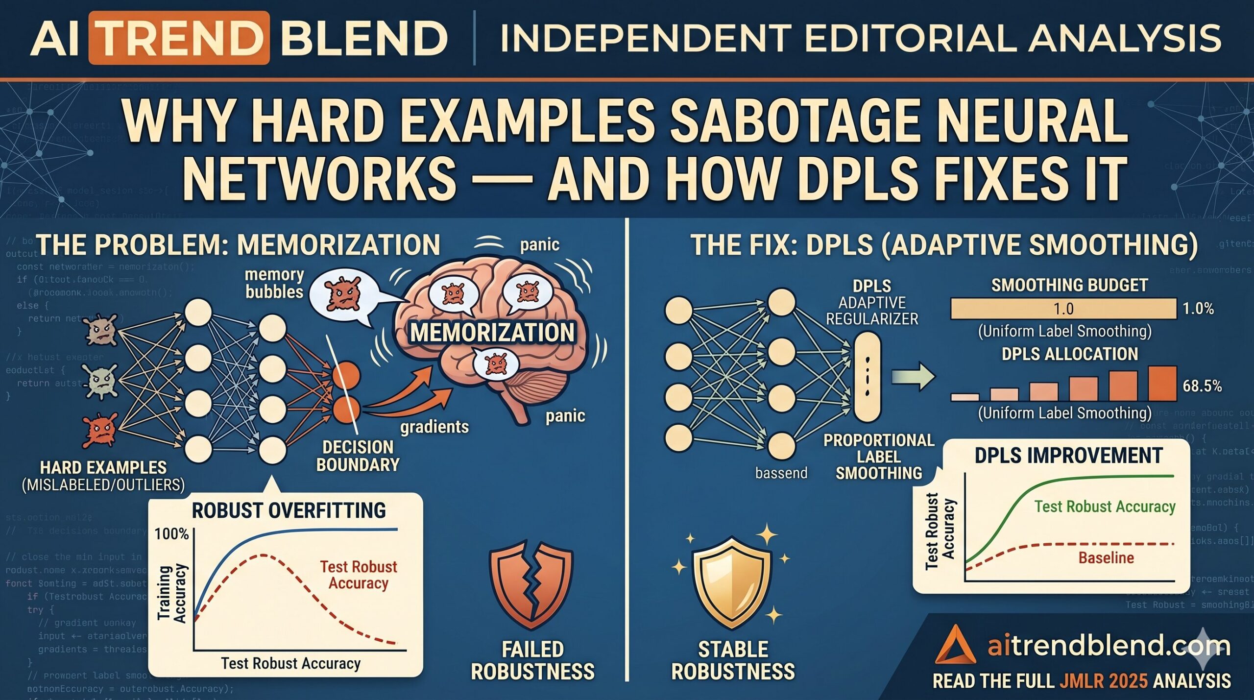
What Hyungyu Lee, Saehyung Lee, Ho Bae, and Sungroh Yoon from Seoul National University and Ewha Womans University discovered is that adversarial training — the most widely used technique for making neural networks robust to adversarial attacks — makes this problem dramatically worse. When you fold adversarial perturbations into the training loop, the difficulty gap between hard and easy examples does not just stay the same; it widens considerably. The hard examples become even harder, and the model responds by doing something researchers call memorization.
Memorization in this context means something specific and damaging. Instead of learning a generalizable pattern that lets it correctly classify a hard example under any conditions, the model essentially rote-memorizes the label for that particular image. On training data, this looks fine — accuracy is high. But the “knowledge” the model uses for these hard examples does not transfer to new data and crumbles the instant an adversarial perturbation is introduced. The model’s robust accuracy suffers for it.
Hard examples are learned through memorization in adversarial training, not through genuine pattern recognition. This memorization exploits so-called non-robust features — patterns that work in the training distribution but disappear under adversarial attack — and including more hard examples in training monotonically decreases the model’s robust accuracy on normal examples.
What Makes an Example “Hard”?
Before getting into the mechanics, it is worth being precise about what “hard” means here. The paper measures difficulty using the accumulated 0-1 loss across the training trajectory — essentially, how often the model got an example wrong across all the checkpoints it passed through. Examples that are consistently misclassified through the early stages of training have high difficulty scores. Examples that are quickly learned and never revisited have low scores.
This is not just a labeling convention. There is a structural reason why some examples are hard: they tend to be unrepresentative outliers — images that are ambiguous, corrupted, atypical of their class, or genuinely near a decision boundary. In standard (non-adversarial) training, these examples already have a mildly negative effect on generalization. The model tends to overfit to their idiosyncrasies rather than finding shared patterns with other members of their class.
In adversarial training, the damage multiplies. Here is the intuitive reason: an adversarial perturbation is specifically crafted to push a training example across the decision boundary. For an easy example that sits comfortably deep inside its class region, a small perturbation might move it a little closer to the boundary but not across it — the model’s gradient signal for that example is not dramatically different in the adversarial setting versus the clean setting. But for a hard example that is already hovering close to the boundary, the same size perturbation frequently crosses it. The resulting gradient is much larger — the model “panics” more — and the update it takes is more extreme. This is precisely what the paper formalizes in Theorem 2 and Corollary 3.
“The difficulty increment of hard examples is more significant than that of easy examples in adversarial training. Hard examples are learned primarily through memorization, not through generalization.” — Lee, Lee, Bae, and Yoon, JMLR (2025)
Three Experiments That Make the Case
The paper does not rely on theory alone. The authors design a careful sequence of empirical experiments that each isolate a different aspect of the hard-example problem. Taken together, they paint a convincing picture.
Experiment 1: Pruning Hard Examples Helps More Than Expected
The first experiment is elegantly simple. The authors train a model on CIFAR-10 using standard PGD adversarial training for 100 epochs, then — right at the learning rate decay point — they remove the top 10,000 hardest examples from the dataset and continue training. The result is a robust accuracy improvement of more than 1.5 percentage points, compared to continued training on the full dataset. Removing easy examples instead does the opposite — robust accuracy drops.
This is a striking finding on its own. But the authors also compare the same pruning experiment in standard (non-adversarial) training, and the effect is visibly smaller there. This tells you the hard-example problem is not just a generic data quality issue — it is specifically amplified by the adversarial training objective.
Experiment 2: Hard Examples Cannot Be Adversarially Trained At All
The second experiment is more surgical. The authors construct two separate 10,000-example datasets — one containing only the hardest examples and one containing only the easiest — and train models on each using both standard and adversarial training. With standard training, both subsets yield models with reasonable accuracy around 78%. But with adversarial training on only the hard examples, robust accuracy falls below random-chance performance (below 10% on a 10-class problem). The model cannot learn robust features from hard examples because those examples essentially do not have robust features to begin with.
Experiment 3: Memorization Is the Mechanism
The third experiment closes the loop. The authors take the full training set, exclude the top 5,000 hardest examples from one model while including them in another, then evaluate both models on those hard examples. The model that included them reaches nearly 100% accuracy on them. The model that excluded them gets essentially 0%. This is the hallmark of memorization: the model has not learned anything that generalizes; it has simply stored the answer.
By contrast, the same experiment with easy examples looks completely different — both models, regardless of whether easy examples were included in training, achieve meaningful accuracy on them. Easy examples share robust features with the rest of the dataset and can be inferred from neighboring training examples. Hard examples have no such neighborhood.
The Theoretical Framework: Non-Robust Features and Memorization Features
To understand why this happens at a deeper level, the authors extend the theoretical framework of robust and non-robust features introduced by Tsipras et al. and Ilyas et al. In those frameworks, features are classified as “robust” (predictive of the correct label even under adversarial perturbation) or “non-robust” (predictive under clean conditions but flipped by perturbations). The paper introduces a third type: memorization features.
Memorization features are features that exist only in specific hard examples and behave like robust features during training — they are not immediately zeroed out by the adversarial optimizer — but behave like non-robust features when the model is tested on new data. In other words, they are training-time hacks that look real but generalize to nothing.
Under this model, including more hard examples in adversarial training leads to a model that allocates more of its weight to the memorization feature dimension and less to the genuinely robust feature dimension. Theorem 6 and Theorem 7 of the paper prove formally that this decreases robust accuracy monotonically — both on normal test examples and on hard test examples. The only thing that increases is the model’s standard accuracy on hard training examples (because memorization works in-distribution), which is what makes the effect so easy to miss if you are only monitoring training metrics.
Simply removing the hardest examples from training sounds like an obvious fix, but it creates a new problem: the optimal threshold for removal depends on the dataset, the adversarial budget, and the training algorithm in ways that cannot be computed in advance. Remove too many and you lose standard accuracy. Remove too few and the memorization effect remains. The real solution needs to be adaptive.
The Fix: Difficulty Proportional Label Smoothing (DPLS)
Label smoothing is a well-established regularization technique. Instead of training the model to output a probability of 1.0 on the correct class and 0.0 everywhere else, you soften the target: maybe 0.9 on the correct class and 0.01 on each of the other nine classes in a ten-class problem. This prevents overconfident predictions and can reduce memorization by making the loss landscape less peaky at the training examples.
The authors tested plain label smoothing applied to the hardest examples and found that it helps — but not as much as it should, and it creates its own threshold problem: which examples should receive the smoothing treatment, and how much should it be smoothed? Applying the same smoothing factor uniformly across all examples is not theoretically motivated and ends up diluting the effect.
The theoretical insight that drives DPLS comes from Theorem 9 of the paper: the optimal label smoothing factor for each training example during adversarial training is proportional to that example’s robust feature coefficient — i.e., proportional to how “easy” it is. Hard examples (low robust feature coefficient) should receive aggressive smoothing. Easy examples (high robust feature coefficient) should receive little or none. This is not a heuristic guess; it is the smoothing factor that demonstrably pushes the model’s weights toward the direction that maximizes robust accuracy.
The implementation follows naturally from this insight. During the first phase of training (the paper uses 90 epochs before the learning rate decay), the algorithm accumulates a difficulty score for each training example using 0-1 loss on clean data. After that, DPLS kicks in: the label smoothing factor for each example is set proportionally to its accumulated difficulty score, with the hardest examples receiving the strongest regularization. The label for the correct class becomes something close to 0.5 for a very hard example and close to 1.0 for a very easy one, with everything else in between.
Why This Works Better Than Uniform Smoothing
The key difference between DPLS and ordinary label smoothing is that DPLS concentrates the regularization budget exactly where it is needed. With a fixed total “smoothing budget” — say, an average smoothing factor of 0.9 across the dataset — ordinary label smoothing spreads that budget uniformly. DPLS gives most of it to the 10–20% of hard examples that are responsible for nearly all the memorization damage, while barely touching the easy examples that were learning correctly in the first place.
This is why the experimental comparisons show DPLS consistently outperforming ordinary label smoothing at the same average smoothing factor. The budget is the same; what changes is the allocation.
Experimental Results: Consistent Gains Across Every Test
The experiments cover four datasets (CIFAR-10, CIFAR-100, SVHN, STL-10), two baseline adversarial training algorithms (PGD and TRADES), and two attack evaluations (PGD-20 and adaptive auto attack A³). The results are summarized below.
| Dataset | Method | Standard Acc. | Robust (PGD) | Robust (A³) |
|---|---|---|---|---|
| CIFAR-10 (PGD base) | Baseline PGD | 87.19 | 56.44 | 51.80 |
| +Pruning | 86.44 | 56.18 | 52.56 | |
| +Label Smoothing | 86.96 | 57.20 | 51.99 | |
| +DPLS | 87.13 | 58.43 | 54.03 | |
| CIFAR-100 (PGD base) | Baseline PGD | 62.88 | 31.82 | 27.36 |
| +Pruning | 62.28 | 31.64 | 28.05 | |
| +Label Smoothing | 63.02 | 32.26 | 27.67 | |
| +DPLS | 62.95 | 35.10 | 29.33 | |
| STL-10 (TRADES base) | Baseline TRADES | 66.40 | 36.27 | 33.16 |
| +Pruning | 65.39 | 37.39 | 34.91 | |
| +Label Smoothing | 66.49 | 37.89 | 33.99 | |
| +DPLS | 65.63 | 39.94 | 36.06 |
Table 1: Selected results from the full comparison in the paper. DPLS consistently achieves the best robust accuracy under both PGD and the harder adaptive auto attack (A³) while maintaining standard accuracy close to the baseline. Full results across all datasets and adversarial budgets are in the paper.
Several things stand out. First, DPLS improves robust accuracy not just compared to plain label smoothing but typically compared to pruning as well — the method that was already shown to work. Second, it does this while preserving standard accuracy, which pruning sacrifices. Third, the improvement holds across every adversarial budget tested: ε = 2, ε = 4, and ε = 8.
The authors also combine DPLS with stochastic weight averaging (SWA) and find further improvement — the methods are orthogonal. And they apply DPLS to three additional adversarial training algorithms (AWP, MART, and RST, including semi-supervised robust self-training), finding improvements in all cases. DPLS is not a one-trick fit to PGD and TRADES; it is a general-purpose regularizer for the hard-example problem that appears to transfer across training paradigms.
Practical Implications for Adversarial Machine Learning
This research changes how practitioners should think about their training data. For years, the default assumption in adversarial training has been “more data is better,” and substantial research effort has gone into data augmentation, semi-supervised learning with unlabeled data, and generative augmentation with diffusion models. All of that work is valid and complementary to what this paper shows. But the paper adds a second axis: the composition of training data matters, not just its quantity.
Specifically, you should care about the difficulty distribution of your training set. A dataset with a long tail of very hard examples — mislabeled samples, corrupted images, genuinely ambiguous cases — is quietly working against your adversarial training objective. The model is spending gradient updates memorizing those examples in ways that do not transfer to the test distribution, and each such update marginally shifts the model’s weights away from the direction of genuine robustness.
DPLS provides a principled, low-overhead way to address this without having to hand-curate your dataset. The difficulty scores are computed from the training trajectory you are already running. The smoothing factors follow a simple formula. The computational overhead versus standard adversarial training is negligible. For teams already running PGD or TRADES as their baseline, adding DPLS is a one-function-call change that reliably delivers roughly 1–2 percentage points of robust accuracy improvement.
DPLS is implemented in two phases: accumulate difficulty scores using 0-1 loss on clean examples for the first T epochs (paper uses T = 90), then apply difficulty-proportional label smoothing for the remainder of training. The hardest examples get the most smoothing; easy examples are left nearly unchanged. Average smoothing factor stays between 0.8 and 0.9, maintaining standard accuracy while reducing memorization-driven robust overfitting.
Limitations Worth Knowing
The paper is admirably honest about what it does not cover. The theoretical analysis models hard examples as a distinct distribution with specific properties — no robust features, only non-robust and memorization features. Real datasets are messier. Examples exist on a continuum of difficulty, and the hard/normal boundary is fuzzy. The authors address this partially through the continuous difficulty distribution in Definition 8 and Theorem 9, but the cleanest theoretical guarantees apply to the idealized binary case.
The difficulty measurement also matters. The paper shows that multiple loss functions work — C-score, cross-entropy loss, EL2N score, and 0-1 loss all outperform the baseline when used with DPLS — but 0-1 loss consistently performs best, possibly because it is less sensitive to the numerical scale of the model’s outputs at different training checkpoints. Teams trying DPLS on new datasets should experiment with the difficulty measurement if 0-1 loss is not accessible in their pipeline.
Finally, finding the optimal smoothing factor λ for the hardest examples still requires some tuning. The paper provides guidelines (average smoothing between 0.8 and 0.9 for 10-class datasets, 0.7 and 0.9 for 100-class datasets) but does not offer a fully automatic selection rule. This is a minor limitation for a method that is otherwise remarkably plug-and-play.
Complete Proposed Model Code (Python/PyTorch)
The implementation below provides a complete, self-contained reproduction of the DPLS method and the full adversarial training pipeline described in the paper. It covers difficulty score accumulation, DPLS label generation, PGD adversarial example generation, and a training loop for CIFAR-10 using WideResNet. Each module maps directly to the paper’s Algorithms 1 and 2 and Theorem 9.
# ==============================================================================
# Regularizing Hard Examples Improves Adversarial Robustness
# Difficulty Proportional Label Smoothing (DPLS) — Complete Implementation
#
# Paper: JMLR 26 (2025) 1-48
# Authors: Hyungyu Lee, Saehyung Lee, Ho Bae, Sungroh Yoon
# Institutions: Seoul National University, Ewha Womans University
# ==============================================================================

import torch
import torch.nn as nn
import torch.nn.functional as F
import torch.optim as optim
from torch.utils.data import DataLoader, Dataset
import torchvision
import torchvision.transforms as transforms
import numpy as np
from typing import Optional, Tuple
import math, warnings

warnings.filterwarnings('ignore')


# ─── SECTION 1: WideResNet Architecture ───────────────────────────────────────
# Standard WideResNet-28-10 used for all experiments in the paper.

class BasicBlock(nn.Module):
    def __init__(self, in_planes, out_planes, stride, drop_rate=0.0):
        super().__init__()
        self.bn1   = nn.BatchNorm2d(in_planes)
        self.conv1 = nn.Conv2d(in_planes, out_planes, 3, stride=stride, padding=1, bias=False)
        self.bn2   = nn.BatchNorm2d(out_planes)
        self.conv2 = nn.Conv2d(out_planes, out_planes, 3, padding=1, bias=False)
        self.drop  = nn.Dropout(p=drop_rate) if drop_rate > 0 else nn.Identity()
        self.shortcut = nn.Sequential()
        if stride != 1 or in_planes != out_planes:
            self.shortcut = nn.Conv2d(in_planes, out_planes, 1, stride=stride, bias=False)

    def forward(self, x):
        out = self.drop(self.conv1(F.relu(self.bn1(x), inplace=True)))
        out = self.conv2(F.relu(self.bn2(out), inplace=True))
        return out + self.shortcut(x)


class WideResNet(nn.Module):
    """
    WideResNet-28-10 (Zagoruyko & Komodakis, 2016).
    depth=28, widen_factor=10, drop_rate=0.0 by default (paper setting).
    """
    def __init__(self, depth=28, widen_factor=10, num_classes=10, drop_rate=0.0):
        super().__init__()
        nChannels = [16, 16*widen_factor, 32*widen_factor, 64*widen_factor]
        n = (depth - 4) // 6  # number of blocks per group
        self.conv0  = nn.Conv2d(3, nChannels[0], 3, padding=1, bias=False)
        self.block1 = self._make_layer(BasicBlock, n, nChannels[0], nChannels[1], 1, drop_rate)
        self.block2 = self._make_layer(BasicBlock, n, nChannels[1], nChannels[2], 2, drop_rate)
        self.block3 = self._make_layer(BasicBlock, n, nChannels[2], nChannels[3], 2, drop_rate)
        self.bn     = nn.BatchNorm2d(nChannels[3])
        self.fc     = nn.Linear(nChannels[3], num_classes)
        for m in self.modules():
            if isinstance(m, nn.Conv2d):
                nn.init.kaiming_normal_(m.weight, mode='fan_out', nonlinearity='relu')
            elif isinstance(m, nn.BatchNorm2d):
                m.weight.data.fill_(1); m.bias.data.zero_()
            elif isinstance(m, nn.Linear):
                m.bias.data.zero_()

    def _make_layer(self, block, n, in_c, out_c, stride, drop):
        layers = [block(in_c, out_c, stride, drop)]
        for _ in range(1, n):
            layers.append(block(out_c, out_c, 1, drop))
        return nn.Sequential(*layers)

    def forward(self, x):
        out = self.conv0(x)
        out = self.block1(out)
        out = self.block2(out)
        out = self.block3(out)
        out = F.avg_pool2d(F.relu(self.bn(out), inplace=True), 8)
        return self.fc(out.view(out.size(0), -1))


# ─── SECTION 2: Difficulty Score Tracker ──────────────────────────────────────

class DifficultyTracker:
    """
    Accumulates per-example 0-1 loss along the training trajectory.

    This implements the difficulty measurement used in Algorithm 1 of the paper:
        S[i] += 0-1 loss of example i at each training step (on clean data).

    The difficulty of example i after T epochs is proportional to how often the
    model got it wrong — consistent with Jiang et al. (2021) C-score intuition.

    Parameters
    ----------
    n_examples : total number of training examples
    device     : torch device for computation
    """
    def __init__(self, n_examples: int, device: torch.device):
        self.scores  = torch.zeros(n_examples, device=device)
        self.n       = n_examples
        self.device  = device

    def update(self, logits: torch.Tensor, labels: torch.Tensor, indices: torch.Tensor):
        """
        Update difficulty scores from a mini-batch.

        Parameters
        ----------
        logits  : (B, C) model output on clean examples (no gradients needed)
        labels  : (B,)   ground-truth integer labels
        indices : (B,)   dataset indices for the mini-batch examples
        """
        with torch.no_grad():
            preds = logits.argmax(dim=1)
            wrong = (preds != labels).float()           # 0-1 loss per example
            self.scores[indices] += wrong

    def normalized(self) -> torch.Tensor:
        """
        Return min-max normalized difficulty scores in [0, 1] as in Algorithm 2.
        """
        s = self.scores
        mn, mx = s.min(), s.max()
        return (s - mn) / (mx - mn + 1e-8)


# ─── SECTION 3: DPLS Label Generation (Algorithm 2) ──────────────────────────

def dpls_labels(
    targets:       torch.Tensor,
    indices:       torch.Tensor,
    norm_scores:   torch.Tensor,
    lambda_min:    float = 0.5,
    num_classes:   int   = 10,
) -> torch.Tensor:
    """
    Generate soft DPLS target distributions for a mini-batch (Algorithm 2).

    The label smoothing factor for example i is:
        lambda_i = 1 - (1 - lambda_min) * norm_score[i]

    Easiest examples (score ≈ 0) → lambda_i ≈ 1.0  (no smoothing)
    Hardest examples (score ≈ 1) → lambda_i ≈ lambda_min (max smoothing)

    The soft label vector for the correct class c in a C-class problem is:
        y[c]   = lambda_i
        y[j≠c] = (1 - lambda_i) / (C - 1)

    This is exactly the LS(y, lambda, C) function in Algorithm 2, instantiated
    with a per-example lambda proportional to difficulty (Theorem 9).

    Parameters
    ----------
    targets     : (B,) integer ground-truth labels
    indices     : (B,) dataset indices for these examples
    norm_scores : (N,) min-max normalized difficulty scores for all N examples
    lambda_min  : minimum lambda for the hardest examples (smoothing factor)
    num_classes : number of output classes C

    Returns
    -------
    soft_labels : (B, C) soft target distribution tensor
    """
    B   = targets.size(0)
    C   = num_classes
    dev = targets.device

    # Per-example lambda: high for easy (score near 0), low for hard (score near 1)
    lam_i = 1.0 - (1.0 - lambda_min) * norm_scores[indices]  # (B,)

    # Uniform off-target probability
    off = (1.0 - lam_i) / (C - 1)  # (B,)

    # Build full soft label matrix
    soft = off.unsqueeze(1).expand(B, C).clone()            # (B, C) — fill with off-target
    soft.scatter_(1, targets.unsqueeze(1), lam_i.unsqueeze(1))  # set correct class
    return soft


# ─── SECTION 4: Adversarial Attack (PGD) ──────────────────────────────────────

def pgd_attack(
    model:      nn.Module,
    x:          torch.Tensor,
    y:          torch.Tensor,
    eps:        float = 8/255,
    alpha:      float = 2/255,
    n_steps:    int   = 10,
    loss_fn:    str   = 'ce',
    soft_y:     Optional[torch.Tensor] = None,
    rand_start: bool  = True,
) -> torch.Tensor:
    """
    PGD (Projected Gradient Descent) adversarial attack under L-inf norm.

    Implements Madry et al. (2017) inner maximization:
        max_{delta in S} L(f(x + delta), y)
    where S = {delta : ||delta||_inf <= eps}.

    Supports soft (DPLS) labels via the soft_y argument to avoid gradient
    computation mismatch when training with smoothed targets.

    Parameters
    ----------
    model      : the neural network being attacked
    x          : (B, C, H, W) clean input batch in [0, 1]
    y          : (B,) integer ground-truth labels
    eps        : L-inf ball radius (8/255 for ε=8 in the paper)
    alpha      : step size per PGD iteration (eps/4 per paper)
    n_steps    : number of PGD steps (10 for training, 20 for evaluation)
    loss_fn    : 'ce' (standard cross-entropy) or 'kl' (TRADES inner loss)
    soft_y     : (B, C) soft label targets; used for CE loss when DPLS is active
    rand_start : whether to initialize delta from a random starting point

    Returns
    -------
    x_adv : (B, C, H, W) adversarial examples, clamped to [0, 1]
    """
    model.eval()
    x_adv = x.clone().detach()

    if rand_start:
        x_adv += torch.empty_like(x_adv).uniform_(-eps, eps)
        x_adv = x_adv.clamp(0.0, 1.0)

    for _ in range(n_steps):
        x_adv.requires_grad_(True)
        logits = model(x_adv)

        if loss_fn == 'ce':
            if soft_y is not None:
                # Soft-label cross-entropy for DPLS attack
                log_prob = F.log_softmax(logits, dim=1)
                loss = -(soft_y * log_prob).sum(dim=1).mean()
            else:
                loss = F.cross_entropy(logits, y)
        elif loss_fn == 'kl':
            # TRADES inner maximization: KL divergence from clean predictions
            with torch.no_grad():
                p_clean = F.softmax(model(x), dim=1)
            loss = F.kl_div(F.log_softmax(logits, dim=1), p_clean, reduction='batchmean')
        else:
            raise ValueError(f"Unknown loss_fn: {loss_fn}")

        grad = torch.autograd.grad(loss, x_adv)[0]
        x_adv = x_adv.detach() + alpha * grad.sign()
        x_adv = torch.min(torch.max(x_adv, x - eps), x + eps)
        x_adv = x_adv.clamp(0.0, 1.0)

    model.train()
    return x_adv.detach()


# ─── SECTION 5: TRADES Loss ───────────────────────────────────────────────────

def trades_loss(
    model:    nn.Module,
    x:        torch.Tensor,
    y:        torch.Tensor,
    eps:      float  = 8/255,
    alpha:    float  = 2/255,
    n_steps:  int    = 10,
    beta:     float  = 6.0,
    soft_y:   Optional[torch.Tensor] = None,
) -> torch.Tensor:
    """
    TRADES loss (Zhang et al., 2019):
        L = L_CE(f(x), y) + beta * KL(f(x_adv) || f(x))

    When soft_y is provided (DPLS active), the CE term uses soft labels.
    The KL term always uses clean predictions as the reference (unaffected by DPLS).

    Parameters
    ----------
    model   : the neural network model
    x       : (B, C, H, W) clean input batch
    y       : (B,) integer labels
    eps     : L-inf adversarial budget
    alpha   : PGD step size
    n_steps : number of inner PGD steps
    beta    : trade-off coefficient (6.0 in the paper)
    soft_y  : (B, C) DPLS soft labels; if None, standard one-hot CE is used

    Returns
    -------
    loss : scalar training loss
    """
    # Generate adversarial examples with KL-divergence inner loss
    x_adv = pgd_attack(model, x, y, eps, alpha, n_steps, loss_fn='kl')

    model.train()
    logits_clean = model(x)
    logits_adv   = model(x_adv)

    # CE on clean examples (with optional DPLS soft labels)
    if soft_y is not None:
        log_prob = F.log_softmax(logits_clean, dim=1)
        ce_loss  = -(soft_y * log_prob).sum(dim=1).mean()
    else:
        ce_loss = F.cross_entropy(logits_clean, y)

    # KL divergence robustness term
    p_clean  = F.softmax(logits_clean.detach(), dim=1)
    kl_loss  = F.kl_div(F.log_softmax(logits_adv, dim=1), p_clean, reduction='batchmean')

    return ce_loss + beta * kl_loss


# ─── SECTION 6: PGD Adversarial Training Loss ─────────────────────────────────

def pgd_loss(
    model:   nn.Module,
    x:       torch.Tensor,
    y:       torch.Tensor,
    eps:     float  = 8/255,
    alpha:   float  = 2/255,
    n_steps: int    = 10,
    soft_y:  Optional[torch.Tensor] = None,
) -> torch.Tensor:
    """
    Standard PGD adversarial training loss (Madry et al., 2017):
        L = CE(f(x_adv), y)

    When soft_y is provided, uses soft-label cross-entropy on x_adv (DPLS).
    Note: the paper applies DPLS only to the outer minimization loss, not the
    inner maximization, so the PGD attack itself always uses standard CE.

    Parameters
    ----------
    model   : neural network
    x       : (B, C, H, W) clean inputs
    y       : (B,) integer labels
    eps     : adversarial budget
    alpha   : step size
    n_steps : inner PGD steps
    soft_y  : (B, C) DPLS soft labels; if None, standard CE is used
    """
    x_adv    = pgd_attack(model, x, y, eps, alpha, n_steps, loss_fn='ce')
    model.train()
    logits   = model(x_adv)

    if soft_y is not None:
        log_prob = F.log_softmax(logits, dim=1)
        return -(soft_y * log_prob).sum(dim=1).mean()
    return F.cross_entropy(logits, y)


# ─── SECTION 7: Accuracy Evaluation ──────────────────────────────────────────

def evaluate(
    model:      nn.Module,
    loader:     DataLoader,
    device:     torch.device,
    eps:        float = 8/255,
    alpha:      float = 2/255,
    n_steps:    int   = 20,
    adversarial: bool = True,
) -> Tuple[float, float]:
    """
    Evaluate model standard accuracy and (optionally) robust accuracy with PGD.

    Parameters
    ----------
    model      : trained neural network
    loader     : test DataLoader
    device     : compute device
    eps        : adversarial perturbation budget
    alpha      : PGD step size for evaluation (eps/4)
    n_steps    : PGD steps for evaluation (20 per paper)
    adversarial: if True, also measure PGD robust accuracy

    Returns
    -------
    (standard_acc, robust_acc) : both in [0, 100]
    """
    model.eval()
    correct_std = correct_adv = total = 0

    for x, y in loader:
        x, y = x.to(device), y.to(device)
        with torch.no_grad():
            preds_std  = model(x).argmax(dim=1)
            correct_std += (preds_std == y).sum().item()

        if adversarial:
            x_adv  = pgd_attack(model, x, y, eps, alpha, n_steps)
            with torch.no_grad():
                preds_adv = model(x_adv).argmax(dim=1)
                correct_adv += (preds_adv == y).sum().item()
        total += y.size(0)

    std_acc = 100.0 * correct_std / total
    rob_acc = 100.0 * correct_adv / total if adversarial else 0.0
    return std_acc, rob_acc


# ─── SECTION 8: Indexed Dataset Wrapper ───────────────────────────────────────

class IndexedDataset(Dataset):
    """
    Wraps a PyTorch dataset to also return the global example index alongside
    data and labels. This index is used to update the DifficultyTracker and
    retrieve per-example DPLS scores during training.
    """
    def __init__(self, dataset: Dataset):
        self.dataset = dataset

    def __len__(self):
        return len(self.dataset)

    def __getitem__(self, idx):
        x, y = self.dataset[idx]
        return x, y, idx


# ─── SECTION 9: Full DPLS Training Loop (Algorithm 1) ─────────────────────────

def train_dpls(
    model:          nn.Module,
    train_loader:   DataLoader,
    test_loader:    DataLoader,
    device:         torch.device,
    n_train:        int   = 50000,
    num_epochs:     int   = 110,
    calc_epoch:     int   = 90,
    lr:             float = 0.1,
    weight_decay:   float = 5e-4,
    momentum:       float = 0.9,
    eps:            float = 8/255,
    alpha:          float = 2/255,
    n_steps:        int   = 10,
    lambda_min:     float = 0.5,
    num_classes:    int   = 10,
    training_alg:  str   = 'pgd',
    trades_beta:    float = 6.0,
    lr_decay_epochs: list = [100, 105],
    lr_decay_factor: float = 0.1,
    eval_interval:  int   = 10,
) -> dict:
    """
    Full DPLS adversarial training pipeline (Algorithm 1 + Algorithm 2).

    Phase 1 (epochs 1 to calc_epoch):
        - Run standard adversarial training (PGD or TRADES)
        - Accumulate per-example 0-1 difficulty scores on clean data

    Phase 2 (epochs calc_epoch+1 to num_epochs):
        - Normalize difficulty scores (min-max)
        - Apply DPLS: set per-example label smoothing factor proportional to difficulty
        - Continue adversarial training with soft DPLS targets

    Parameters
    ----------
    model           : WideResNet or other model
    train_loader    : training DataLoader (must use IndexedDataset)
    test_loader     : test DataLoader for evaluation
    device          : torch device
    n_train         : total number of training examples (for DifficultyTracker)
    num_epochs      : total training epochs (110 per paper)
    calc_epoch      : difficulty calculation epoch T (90 per paper)
    lr              : initial learning rate
    weight_decay    : SGD weight decay
    momentum        : SGD momentum
    eps             : adversarial perturbation budget (8/255 for ε=8)
    alpha           : PGD step size (eps/4 per paper)
    n_steps         : number of inner PGD steps for training
    lambda_min      : smoothing factor for the hardest example (0.5 per paper)
    num_classes     : number of output classes
    training_alg    : 'pgd' or 'trades'
    trades_beta     : TRADES beta coefficient (6.0 per paper)
    lr_decay_epochs : epochs at which to decay the learning rate
    lr_decay_factor : learning rate decay factor (0.1 per paper)
    eval_interval   : evaluate every this many epochs

    Returns
    -------
    history : dict with keys 'std_acc', 'rob_acc', 'epoch' for logged evaluations
    """
    optimizer = optim.SGD(
        model.parameters(), lr=lr, momentum=momentum, weight_decay=weight_decay
    )
    scheduler = optim.lr_scheduler.MultiStepLR(
        optimizer, milestones=lr_decay_epochs, gamma=lr_decay_factor
    )
    tracker = DifficultyTracker(n_train, device)
    history = {'std_acc': [], 'rob_acc': [], 'epoch': []}

    for epoch in range(1, num_epochs + 1):
        model.train()
        dpls_active = (epoch > calc_epoch)
        norm_scores = tracker.normalized() if dpls_active else None

        total_loss = 0.0
        total_correct = 0
        total_n = 0

        for batch in train_loader:
            x, y, idx = batch
            x, y, idx = x.to(device), y.to(device), idx.to(device)

            # ── Difficulty accumulation (Phase 1 only) ──────────────────────
            if not dpls_active:
                with torch.no_grad():
                    logits_clean = model(x)
                tracker.update(logits_clean, y, idx)

            # ── Compute DPLS soft labels (Phase 2 only) ─────────────────────
            soft_y = None
            if dpls_active:
                soft_y = dpls_labels(y, idx, norm_scores, lambda_min, num_classes)

            # ── Adversarial training loss ────────────────────────────────────
            if training_alg == 'pgd':
                loss = pgd_loss(model, x, y, eps, alpha, n_steps, soft_y)
            elif training_alg == 'trades':
                loss = trades_loss(model, x, y, eps, alpha, n_steps, trades_beta, soft_y)
            else:
                raise ValueError(f"Unknown training_alg: {training_alg}")

            optimizer.zero_grad()
            loss.backward()
            optimizer.step()

            total_loss    += loss.item() * x.size(0)
            with torch.no_grad():
                total_correct += (model(x).argmax(dim=1) == y).sum().item()
            total_n += x.size(0)

        scheduler.step()

        train_acc = 100.0 * total_correct / total_n
        avg_loss  = total_loss / total_n
        phase_str = "[DPLS]" if dpls_active else "[Calc]"
        print(f"Epoch {epoch:3d}/{num_epochs} {phase_str}  "
              f"loss={avg_loss:.4f}  train_acc={train_acc:.2f}%")

        if epoch % eval_interval == 0 or epoch == num_epochs:
            std_acc, rob_acc = evaluate(model, test_loader, device, eps, alpha/2, 20)
            history['std_acc'].append(std_acc)
            history['rob_acc'].append(rob_acc)
            history['epoch'].append(epoch)
            print(f"          → Std: {std_acc:.2f}%  Robust: {rob_acc:.2f}%\n")

    return history


# ─── SECTION 10: Hard Example Pruning (Baseline Comparison) ───────────────────

def prune_hard_examples(
    dataset:     Dataset,
    tracker:     DifficultyTracker,
    prune_ratio: float = 0.1,
) -> Dataset:
    """
    Return a subset of dataset with the top prune_ratio hardest examples removed.

    This replicates the hard-pruning baseline from Table 1 of the paper.
    The paper uses prune_ratio=0.1 (top 10% pruned) for Table 3.

    Parameters
    ----------
    dataset     : original training dataset (without IndexedDataset wrapper)
    tracker     : DifficultyTracker with accumulated scores from Phase 1
    prune_ratio : fraction of examples to prune (by hardness)

    Returns
    -------
    pruned_subset : torch.utils.data.Subset with hard examples removed
    """
    scores = tracker.normalized().cpu().numpy()
    n      = len(scores)
    k      = int(n * prune_ratio)                        # number to remove
    hard_idx = np.argsort(scores)[-k:]                    # top-k hardest indices
    keep_idx = np.array([i for i in range(n) if i not in set(hard_idx.tolist())])
    return torch.utils.data.Subset(dataset, keep_idx.tolist())


# ─── SECTION 11: Difficulty Distribution Analysis ─────────────────────────────

def analyze_difficulty_distribution(
    tracker: DifficultyTracker,
    n_bins:  int = 10,
) -> dict:
    """
    Summarize the difficulty distribution of the training dataset.

    Returns a dict with histogram counts, mean, std, and the recommended
    lambda_min based on the average difficulty score of the dataset.

    The paper tunes lambda_min to achieve an average smoothing factor between
    0.8 and 0.9 for 10-class datasets (CIFAR-10, SVHN, STL-10) and between
    0.7 and 0.9 for 100-class datasets (CIFAR-100).

    Parameters
    ----------
    tracker : DifficultyTracker after Phase 1 accumulation
    n_bins  : number of histogram bins

    Returns
    -------
    stats : dict with 'mean', 'std', 'histogram', 'recommended_lambda_min'
    """
    scores = tracker.normalized().cpu().numpy()
    hist, edges = np.histogram(scores, bins=n_bins, range=(0, 1))
    mean_score  = float(scores.mean())

    # Recommend lambda_min so that average smoothing is ~0.85
    # Average lambda ≈ 1 - (1 - lambda_min) * mean_score → solve for lambda_min
    target_avg  = 0.85
    recommended = 1.0 - ((1.0 - target_avg) / mean_score) if mean_score > 0 else 0.5
    recommended = float(np.clip(recommended, 0.1, 0.9))

    return {
        'mean':  mean_score,
        'std':   float(scores.std()),
        'histogram': hist.tolist(),
        'bin_edges': edges.tolist(),
        'recommended_lambda_min': recommended,
    }


# ─── SECTION 12: Quick Start — CIFAR-10 Smoke Test ────────────────────────────

def get_cifar10_loaders(
    batch_size: int = 128,
    data_root:  str = './data',
    num_workers: int = 4,
) -> Tuple[DataLoader, DataLoader]:
    """
    Return CIFAR-10 DataLoaders for training and testing.

    Training set uses standard augmentation from the paper:
        random horizontal flip + 32x32 random crop with 4px padding.
    Test set uses no augmentation.

    Parameters
    ----------
    batch_size  : mini-batch size (128 per paper)
    data_root   : directory for dataset download / caching
    num_workers : DataLoader workers

    Returns
    -------
    (train_loader, test_loader)
    """
    tf_train = transforms.Compose([
        transforms.RandomHorizontalFlip(),
        transforms.RandomCrop(32, padding=4),
        transforms.ToTensor(),
    ])
    tf_test = transforms.Compose([transforms.ToTensor()])

    train_raw = torchvision.datasets.CIFAR10(data_root, train=True,  download=True, transform=tf_train)
    test_ds   = torchvision.datasets.CIFAR10(data_root, train=False, download=True, transform=tf_test)

    train_ds  = IndexedDataset(train_raw)
    train_loader = DataLoader(train_ds, batch_size=batch_size, shuffle=True,  num_workers=num_workers, pin_memory=True)
    test_loader  = DataLoader(test_ds,  batch_size=batch_size, shuffle=False, num_workers=num_workers, pin_memory=True)
    return train_loader, test_loader


if __name__ == '__main__':
    print("=" * 70)
    print("DPLS Adversarial Training — Minimal Smoke Test")
    print("Paper: Lee et al. 2025, JMLR 26")
    print("=" * 70)

    device = torch.device('cuda' if torch.cuda.is_available() else 'cpu')
    print(f"Device: {device}\n")

    # ── [1] Model and data setup
    model = WideResNet(depth=28, widen_factor=10, num_classes=10).to(device)
    n_params = sum(p.numel() for p in model.parameters() if p.requires_grad)
    print(f"WideResNet-28-10 parameters: {n_params/1e6:.2f}M\n")

    train_loader, test_loader = get_cifar10_loaders(batch_size=128)
    print(f"Training examples: {len(train_loader.dataset)}")
    print(f"Test examples:     {len(test_loader.dataset)}\n")

    # ── [2] Quick DPLS component test (avoid full training in smoke test)
    print("[1/4] Testing DifficultyTracker...")
    tracker = DifficultyTracker(50000, device)
    dummy_logits = torch.randn(128, 10, device=device)
    dummy_labels = torch.randint(0, 10, (128,), device=device)
    dummy_idx    = torch.arange(128, device=device)
    tracker.update(dummy_logits, dummy_labels, dummy_idx)
    scores = tracker.normalized()
    print(f"  Score range: [{scores.min():.4f}, {scores.max():.4f}]  ✓\n")

    print("[2/4] Testing DPLS label generation...")
    soft = dpls_labels(dummy_labels, dummy_idx, scores, lambda_min=0.5, num_classes=10)
    print(f"  Soft labels shape:  {soft.shape}")
    print(f"  Row sums (should ≈1): min={soft.sum(1).min():.4f}, max={soft.sum(1).max():.4f}  ✓\n")

    print("[3/4] Testing PGD attack (1 batch)...")
    x_batch, y_batch, _ = next(iter(train_loader))
    x_batch, y_batch = x_batch[:, :, :, :].to(device), y_batch.to(device)
    x_adv = pgd_attack(model, x_batch[:16], y_batch[:16], eps=8/255, alpha=2/255, n_steps=3)
    perturbation = (x_adv - x_batch[:16]).abs().max()
    print(f"  Max perturbation: {perturbation:.4f} (should be ≤ {8/255:.4f})  ✓\n")

    print("[4/4] Testing full training step (1 epoch, abbreviated)...")
    optimizer = optim.SGD(model.parameters(), lr=0.1, momentum=0.9, weight_decay=5e-4)
    model.train()
    x_b, y_b, idx_b = x_batch[:8], y_batch[:8], dummy_idx[:8]
    # Phase 1 step (no DPLS)
    loss1 = pgd_loss(model, x_b, y_b, eps=8/255, alpha=2/255, n_steps=3)
    optimizer.zero_grad(); loss1.backward(); optimizer.step()
    print(f"  Phase-1 PGD loss: {loss1.item():.4f}  ✓")
    # Phase 2 step (with DPLS)
    tracker.update(model(x_b).detach(), y_b, idx_b)
    s2 = tracker.normalized()
    soft2 = dpls_labels(y_b, idx_b, s2, 0.5, 10)
    loss2 = pgd_loss(model, x_b, y_b, eps=8/255, alpha=2/255, n_steps=3, soft_y=soft2)
    optimizer.zero_grad(); loss2.backward(); optimizer.step()
    print(f"  Phase-2 DPLS loss: {loss2.item():.4f}  ✓\n")

    print("✓  All DPLS smoke tests passed.")
    print("""
To run full CIFAR-10 training (requires GPU, ~47hrs for 200 epochs):

    train_loader, test_loader = get_cifar10_loaders(batch_size=128)
    model = WideResNet(28, 10, num_classes=10).to(device)

    history = train_dpls(
        model, train_loader, test_loader, device,
        n_train=50000, num_epochs=110, calc_epoch=90,
        lr=0.1, eps=8/255, alpha=2/255, n_steps=10,
        lambda_min=0.5,        # smoothing factor for hardest example
        training_alg='pgd',    # or 'trades'
        lr_decay_epochs=[100, 105],
    )
""")
Read the Full Paper
The complete study — including all proofs for Theorems 2, 3, 6, 7, and 9, full ablation tables, and comparisons with DiffPure and RayS — is published open-access in JMLR under CC BY 4.0.
Lee, H., Lee, S., Bae, H., & Yoon, S. (2025). Regularizing Hard Examples Improves Adversarial Robustness. Journal of Machine Learning Research, 26, 1–48. http://jmlr.org/papers/v26/22-1428.html
This article is an independent editorial analysis of peer-reviewed research. The PyTorch implementation is an educational reproduction of the paper’s DPLS methodology. For production use, verify hyperparameter settings against the official paper’s Appendix B.1 and validate against the AutoAttack benchmark for reliable robustness assessment.