When Matrices Draw Ellipses — The Hidden Geometry of Higher Rank Numerical Ranges

Three Portuguese mathematicians have proved that a sweeping family of block matrices produces higher rank numerical ranges with a strikingly clean shape — perfect elliptical discs — and along the way unified dozens of scattered results under a single elegant framework with direct consequences for quantum error correction.

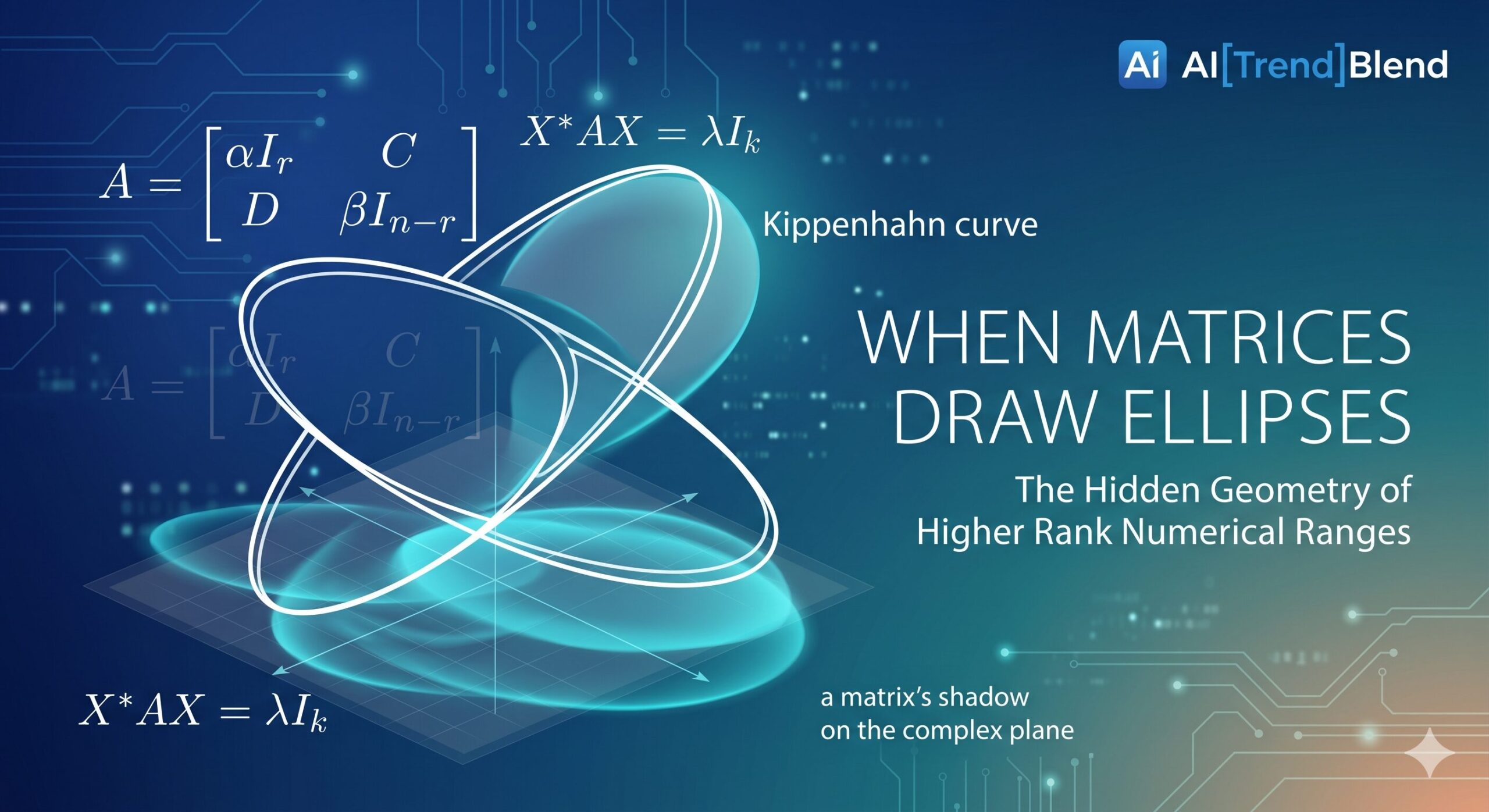
Picture drawing the “shadow” of a matrix — not its spectrum, but the full cloud of values it can produce when paired with unit vectors. For most matrices, that cloud is a complicated convex shape. For a 2×2 matrix, it is always an ellipse. The question that has occupied matrix theorists for decades is: when does this elliptical simplicity survive as matrices grow larger and more structured? A new paper from three Portuguese universities gives the most comprehensive answer yet — and the consequences reach from abstract linear algebra all the way to the practical problem of protecting quantum information from errors.

The Numerical Range — A Matrix’s Shadow on the Complex Plane

Every matrix has a spectrum — the set of its eigenvalues. But eigenvalues alone do not tell the full story of how a matrix behaves. The numerical range of a matrix \(A\), written \(W(A)\), captures something richer: it is the set of all values of the form \(\langle Ax, x \rangle\) as the unit vector \(x\) ranges over the entire space. Formally,

This set — introduced independently by Toeplitz in 1918 and Hausdorff in 1919 — is always convex, always contains the spectrum of \(A\), and carries a wealth of geometric information about how \(A\) acts. For a 2×2 matrix with eigenvalues \(\lambda_1\) and \(\lambda_2\), the classical Elliptical Range Theorem guarantees that \(W(A)\) is always an elliptical disc. The foci sit at the eigenvalues; the axis lengths are determined by the matrix entries. Clean. Predictable. Elegant.

The problem runs deeper when you try to generalize. For larger matrices, \(W(A)\) can be far more irregular. Researchers have known for years that certain structured matrix classes — tridiagonal matrices with special periodicity, block matrices with particular symmetry between off-diagonal blocks — retain elliptical numerical ranges regardless of size. But these results accumulated piecemeal over decades, each proved by different authors with different techniques, making it difficult to see the underlying pattern.

Rank-k Numerical Ranges — Born From Quantum Error Correction

The story does not stop with the classical numerical range. In 2006, Choi, Kribs, and Życzkowski introduced a family of generalizations for a specific purpose: understanding compression in quantum error correction. The rank-\(k\) numerical range of a matrix \(A \in M_n\) is defined as

The rank-1 case recovers the classical \(W(A)\). For \(k > 1\), these sets ask a harder question: can you compress the matrix \(A\) into a scalar multiple of the identity on some \(k\)-dimensional subspace? The answer — and the shape of the resulting set in the complex plane — determines whether quantum error correction is possible on that subspace.

The sets \(\Lambda_k(A)\) form a decreasing sequence: \(\Lambda_n(A) \subseteq \cdots \subseteq \Lambda_1(A) = W(A)\). As \(k\) grows, the sets shrink. For \(k > n/2\), each \(\Lambda_k(A)\) is either empty or a single point — an eigenvalue of \(A\) with high geometric multiplicity. Li, Poon, and Sze proved that \(\Lambda_k(A)\) is non-empty whenever \(k < n/3 + 1\). The difficult, practically important regime is everything in between: when is \(\Lambda_k(A)\) an ellipse, and which ellipse?

That is precisely what N. Bebiano (University of Coimbra), R. Lemos (University of Aveiro), and G. Soares (University of Trás-os-Montes e Alto Douro) set out to answer in their new paper, published in the Journal of Mathematical Analysis and Applications in March 2026.

The Kippenhahn Curve — Reading a Matrix’s Geometry

Before the main results can be stated, one more piece of background is essential: the Kippenhahn curve. In 1951, Rudolf Kippenhahn proved that the boundary of \(W(A)\) is the convex hull of a specific algebraic curve \(C(A)\) attached to the matrix — now called the Kippenhahn curve. This curve is the envelope of the family of tangent lines to \(W(A)\), parametrized by angle.

Here is where it gets interesting. The Kippenhahn curve does not have to be a single connected piece. For many structured matrices — particularly block matrices where the off-diagonal blocks have special relationships — the curve \(C(A)\) splits into several elliptical components. Each component is an ellipse. The numerical range \(W(A)\) is then the convex hull of those ellipses, and the rank-\(k\) numerical range \(\Lambda_k(A)\) can be described as intersections of convex hulls of subsets of those ellipses.

The key structural insight that drives this paper is that when the Hermitian matrix \(\text{Re}(e^{-i\theta}A)\) — formed by rotating \(A\) by angle \(\theta\) and taking the real part — decomposes into a direct sum of 2×2 blocks for every \(\theta\), the Kippenhahn curve automatically splits into elliptical pieces. Each 2×2 block contributes one ellipse to \(C(A)\). The entire problem of characterizing \(\Lambda_k(A)\) then reduces to understanding which ellipses appear and how they nest.

The Block Matrix Framework — What the Paper Studies

The matrices Bebiano, Lemos, and Soares study have the specific 2×2 block structure

where \(\alpha\) and \(\beta\) are complex scalars, and \(C\), \(D\) are rectangular matrices forming the off-diagonal blocks. This structure is broad. Tridiagonal matrices with biperiodic diagonals, arrowhead matrices, shift operators, quadratic matrices — all of them can be written or permuted into this form. The diagonal blocks are scalar multiples of the identity, which is the structural constraint that makes things tractable.

The critical quantity for the analysis is a matrix \(M_{C,D}(\theta)\) defined by

The eigenvalues of this matrix control the eigenvalues of \(\text{Re}(e^{-i\theta}A)\) — and therefore the shape of the Kippenhahn curve. When the eigenvalues of \(M_{C,D}(\theta)\) can be explicitly tracked as functions of \(\theta\), the geometry of the numerical range becomes computable.

The central structural lemma of the paper — Lemma 2.1 — shows that the matrix \(\text{Re}(e^{-i\theta}B)\), where \(B = A – \frac{1}{2}(\alpha + \beta)I_n\), is always unitarily similar to a direct sum of 2×2 blocks \(B_j\) of the form

where \(w_\theta = \text{Re}(we^{-i\theta})\), \(w = (\alpha – \beta)/2\), and \(s_j(\theta)\) are the non-zero singular values of the matrix \(N_\theta = \frac{1}{2}(e^{-i\theta}C + e^{i\theta}D^*)\). Each of these 2×2 blocks has eigenvalues \(\pm\sqrt{w_\theta^2 + s_j(\theta)^2}\), which trace out an ellipse as \(\theta\) varies. The Kippenhahn curve of the full matrix is therefore the union of these ellipses — one per non-zero singular value — plus isolated points corresponding to the scalar diagonal blocks.

The Main Theorem — Ellipses, Nesting, and a Complete Description

The main result — Theorem 2.1 — gives a complete characterization of every \(\Lambda_k(A)\) under an explicit condition on the off-diagonal blocks \(C\) and \(D\). The condition is that the matrix \(DC\) is normal and commutes with \(C^*C + DD^*\). When this holds, those two matrices can be simultaneously diagonalized by the same unitary transformation — a standard algebraic fact — and everything simplifies.

This is a strikingly complete answer. Every rank-\(k\) numerical range, for every value of \(k\) from 1 to \(n – r\), is given by an explicit intersection formula involving only convex hulls of known ellipses. There is no residual mystery about the shape: once you know the eigenvalues \(z_j\) and \(h_j\), you know everything about every \(\Lambda_k(A)\).

What makes this especially satisfying is the nesting behavior. When the elliptical discs \(\mathcal{E}_j\) bounded by \(\hat{\mathcal{E}}_j\) form a nested chain — \(\mathcal{E}_{n-r} \subseteq \cdots \subseteq \mathcal{E}_1\) — the intersection formula collapses entirely, giving the beautifully clean result \(\Lambda_k(A) = \mathcal{E}_k\). Each rank-\(k\) numerical range is simply the \(k\)-th elliptical disc in the chain. No intersections to compute. No convex hulls to take.

“The boundary generating curve of \(W(A)\) splits into at most \(n/2\) elliptical components, each solely responsible for the respective higher rank numerical range — a structural decomposition that makes the entire hierarchy of rank-k ranges readable at once.” — Bebiano, Lemos, Soares · J. Math. Anal. Appl. 560 (2026)

Three Corollaries That Unify a Decade of Scattered Results

The real payoff of Theorem 2.1 is its reach. The authors derive a sequence of corollaries that recover — in a unified, elementary way — results that previously required separate proofs, separate techniques, and sometimes significant computation.

Arrowhead Matrices

An arrowhead matrix has a single scalar entry \(\alpha\) repeated on all-but-one diagonal positions, with the remaining row and column forming a “head” at one corner. These matrices appear naturally in eigenvalue computations and data science. Corollary 3.3 shows that for any arrowhead matrix of size \(n \geq 3\), the rank-1 numerical range \(\Lambda_1(A) = W(A)\) is a single elliptical disc, the rank-\(k\) range for \(2 \leq k \leq n-1\) collapses to the single point \(\{\alpha\}\) (or \(\{\beta\}\)), and \(\Lambda_n(A)\) is empty. The ellipse’s foci and axes are given explicitly in terms of the arrowhead entries.

Tridiagonal Matrices With Biperiodic Structure

Perhaps the most practically useful application is to tridiagonal matrices. A tridiagonal matrix \(T(d, a, c)\) with biperiodic main diagonal \((\alpha, \beta, \alpha, \beta, \ldots)\) and off-diagonals satisfying a proportionality condition \(c_j = \zeta d_j\) on a subset of indices arises in discretizations of differential operators, Jacobi matrices from orthogonal polynomial theory, and tight-binding models in condensed matter physics. Corollary 3.5 gives the rank-\(k\) numerical range of any such matrix in terms of the singular values of an associated bidiagonal matrix \(B(\tilde{c})\) — computable directly from the entries.

One immediate consequence: the rank-\(k\) numerical range of the \(n\)-dimensional shift operator — the matrix with ones on the subdiagonal and zeros elsewhere — is the circular disc centered at the origin with radius \(\cos(k\pi/(n+1))\), for \(1 \leq k \leq \lfloor(n+1)/2\rfloor\). This result, previously known from separate papers by Gaaya and by Poon-Spitkovsky-Woerdeman, now falls out as a one-line corollary.

Theta-Independent Spectrum — A Cleaner Special Case

Theorem 3.1 handles an independent special case: matrices where the spectrum of \(M_{C,D}(\theta)\) does not depend on \(\theta\) at all. When this holds, the Kippenhahn curve contains only ellipses that share the same foci — at \(\alpha\) and \(\beta\) — with minor axes equal to the singular values of \(C + D^*\). The whole range hierarchy \(\Lambda_k(A) = E(\alpha, \beta; s_k)\) follows immediately, where \(E(\alpha, \beta; s)\) denotes the elliptical disc with foci at \(\alpha\) and \(\beta\) and minor axis \(s\). This covers quadratic matrices — matrices with a minimal polynomial of degree two — as a direct special case.

A Worked Example — Seeing the Nesting in Action

The paper includes a concrete 6×6 example that illustrates the theory vividly. The matrix in question has \(\alpha = 2\), \(\beta = 3\), and off-diagonal blocks with entries that at first glance look quite irregular. Yet the analysis shows that its non-empty higher rank numerical ranges \(\Lambda_1(A)\), \(\Lambda_2(A)\), and \(\Lambda_3(A)\) form a perfectly nested chain of three elliptical discs — each contained inside the previous one, sharing the same center.

The authors visualize this in Figure 3.1 of the paper: three concentric ellipses, drawn in red (\(k = 1\)), blue (\(k = 2\)), and black (\(k = 3\)), with their foci marked. The picture is striking precisely because nothing about the raw matrix entries suggests such regularity. The geometric structure is a consequence of the algebraic conditions — and without the theorem, you would never guess it from the matrix alone.

The Quantum Error Correction Connection

None of this geometry exists in a vacuum. The higher rank numerical range was invented to solve a specific problem in quantum information theory: given a quantum channel (a physical process that introduces noise), on which subspaces can you encode quantum information so that errors can be detected and corrected?

The mathematical formulation is this: a quantum code of dimension \(k\) can correct errors introduced by an operator \(A\) if and only if \(\Lambda_k(A)\) contains the origin — or more precisely, if \(A\) compressed to the code subspace behaves as a scalar. The shape of \(\Lambda_k(A)\) tells you how much freedom you have in choosing such a subspace and how robust the code is to variations in the physical parameters.

When \(\Lambda_k(A)\) is an ellipse — as guaranteed by the results of this paper for block matrices of type (1.3) — the geometry of the error-correction problem becomes tractable. You can explicitly calculate whether the origin lies inside the ellipse, how close the boundary is, and how the code quality degrades as \(k\) increases. For practical quantum computing, where the matrix \(A\) represents the dominant noise source, these are not abstract questions.

The shift operator result is particularly relevant here. Physical quantum systems often have dynamics described by shift-type operators — representing the sequential propagation of quantum information through a chain of qubits. Knowing that the rank-\(k\) numerical range of the \(n\)-dimensional shift is a disc of radius \(\cos(k\pi/(n+1))\) gives immediate, computable bounds on the error-correcting capacity of shift-invariant codes.

What Remains Open — Honest Limits of the Current Results

The paper itself raises two open questions at its close, and they are worth dwelling on. The first asks for necessary and sufficient conditions for elliptical higher rank numerical ranges in the block matrix class (1.3) beyond what Theorems 2.1 and 3.1 cover. The current results require either the normality-commutativity condition or the theta-independence of the spectrum. Example 3.1 shows that ellipticity can occur even when neither condition is met — so something is missing from the theory.

The second open question concerns infinite-dimensional extensions. The paper works throughout with finite \(n \times n\) matrices. But the block structure (1.3), with two scalar infinite diagonal blocks, can be extended to bi-infinite operators. The geometry of numerical ranges for such operators — including the shift on \(\ell^2(\mathbb{Z})\) — is considerably more subtle, and the techniques developed here do not transfer directly.

There is also a limitation that the paper does not explicitly flag but that any careful reader will notice: the commutativity condition \(DC \cdot (C^*C + DD^*) = (C^*C + DD^*) \cdot DC\) is an algebraic condition that is easy to state but not always easy to verify for a given matrix. In practice, checking it may require computing products of large matrices. The paper gives several sufficient conditions — \(DC = zI\), \(D = \zeta C^*\) — that guarantee commutativity automatically, but the gap between these sufficient conditions and the general theorem remains a real constraint on applicability.

Conclusion — Geometry as a Unifying Language

What Bebiano, Lemos, and Soares have accomplished is something that pure mathematics does at its best: they took a landscape of scattered, individually proved results — each with its own notation, its own proof technique, its own level of generality — and found the common geometric structure underneath. The key was not a new computation but a new perspective: approach the problem through the Kippenhahn curve, decompose the rotated Hermitian part into 2×2 blocks via a singular value decomposition, and let the ellipses emerge naturally.

That shift in perspective is more valuable than any single corollary. The corollaries themselves — the shift operator, the arrowhead matrices, the tridiagonal 2-Toeplitz matrices, the quadratic matrices — were already known. What was missing was the understanding of why they all come out elliptical. The answer, it turns out, is the same in every case: the off-diagonal blocks have a special algebraic relationship that forces the Kippenhahn curve to split into ellipses, and the nesting of those ellipses then determines the entire hierarchy of rank-\(k\) ranges.

The quantum error correction connection adds a practical dimension that is easy to underestimate. Matrix theory and quantum information may feel like distant cousins, but the rank-\(k\) numerical range sits precisely at their intersection. When the geometry is clean — when the ranges are ellipses — the error-correction problem becomes analytically tractable. Codes can be designed, boundaries can be computed, and stability can be guaranteed. The results of this paper make that tractability available for a wide class of physically relevant operators.

The two open questions — necessary and sufficient conditions, and the infinite-dimensional extension — point toward a continuing research program. The authors of this paper have been developing the theory of numerical ranges for structured matrices across multiple publications since at least 2021, and the present paper is clearly not a stopping point. A complete characterization of elliptical higher rank numerical ranges for block matrices, without restricting to normal or commuting products, would be a significant achievement — and the framework developed here seems well-positioned to reach it.

There is a broader lesson here, too. Geometry has a way of revealing truth that algebra alone sometimes obscures. The spectrum of a matrix tells you its eigenvalues. The numerical range tells you how the matrix behaves across all unit vectors. The higher rank numerical range tells you what codes are possible. Each layer adds information — and each layer, in the right hands, adds beauty. The ellipses that appear in this paper are not decorative. They are the geometry of what is possible.

References

• [1] M. Adam, A. Aretaki, I.M. Spitkovsky. Elliptical higher rank numerical range of some Toeplitz matrices. Linear Algebra Appl. 549 (2018) 256–275.
• [2] N. Bebiano, J. da Providência. Numerical ranges in physics. Linear Multilinear Algebra 43 (1998) 327–337.
• [3] N. Bebiano, J. da Providência, A. Nata. The numerical range of banded biperiodic Toeplitz operators. J. Math. Anal. Appl. 398 (2013) 189–198.
• [4] N. Bebiano, R. Lemos, J. da Providência. Numerical ranges of unbounded operators arising in quantum physics. Linear Algebra Appl. 381 (2004) 259–279.
• [5] N. Bebiano, S. Furtado. Remarks on anti-tridiagonal matrices. Appl. Math. Comput. 373 (2020) 125008.
• [6] N. Bebiano, S. Furtado. A note on classes of structured matrices with elliptical type numerical range. Czechoslov. Math. J. 71 (4) (2021) 1015–1023.
• [7] N. Bebiano, J. da Providência, I. Spitkovsky, V. Kenya. Kippenhahn curves of some tridiagonal matrices. Filomat 35 (2021) 3047–3061.
• [8] N. Bebiano, J. da Providência, I.M. Spitkovsky. On Kippenhahn curves and higher-rank numerical ranges of some matrices. Linear Algebra Appl. 629 (2021) 246–257.
• [9] M.-D. Choi, D.W. Kribs, K. Życzkowski. Higher-rank numerical ranges and compression problems. Linear Algebra Appl. 418 (2006) 828–839.
• [10] M.-D. Choi, D.W. Kribs, K. Życzkowski. Quantum error correcting codes from the compression formalism. Rep. Math. Phys. 58 (1) (2006) 77–91.
• [11] T. Geryba, I.M. Spitkovsky. On the numerical range of some block matrices with scalar diagonal blocks. Linear Multilinear Algebra 69 (2021) 772–785.
• [12] R. Kippenhahn. Über den Wertevorrat einer Matrix. Math. Nachr. 6 (3–4) (1951) 193–228.
• [13] C.-K. Li, N.-S. Sze. Canonical forms, higher rank numerical ranges, totally isotropic subspaces, and matrix equations. Proc. Am. Math. Soc. 136 (2008) 3013–3023.
• [14] C.K. Li, Y.-T. Poon, N.-S. Sze. Condition for the higher rank numerical range to be non-empty. Linear Multilinear Algebra 57 (4) (2009) 365–368.
• [15] H.J. Woerdeman. The higher rank numerical range is convex. Linear Multilinear Algebra 56 (1–2) (2008) 65–67.
• [16] O. Toeplitz. Das algebraische Analogon zu einem Satze von Fejér. Math. Z. 2 (1918) 187–197.
• [17] F. Hausdorff. Der Wertvorrat einer Bilinearform. Math. Z. 3 (1919) 314–316.