Pinning Down the Zeros — New Uniform Asymptotic Expansions for Generalised Trigonometric Integrals | AI Trend Blend

Applied Mathematics · Journal of Mathematical Analysis and Applications 560 (2026) · San Diego State University · 13 min read

Pinning Down the Zeros — How a Single Elegant Chain of Analysis Finally Tames the Generalised Trigonometric Integrals

A mathematician at San Diego State University has derived powerful new uniform asymptotic expansions for the generalised trigonometric integrals and — for the first time — their zeros, all at once, for every size of zero, using a beautifully layered argument rooted in Liouville-Green theory and incomplete gamma functions.

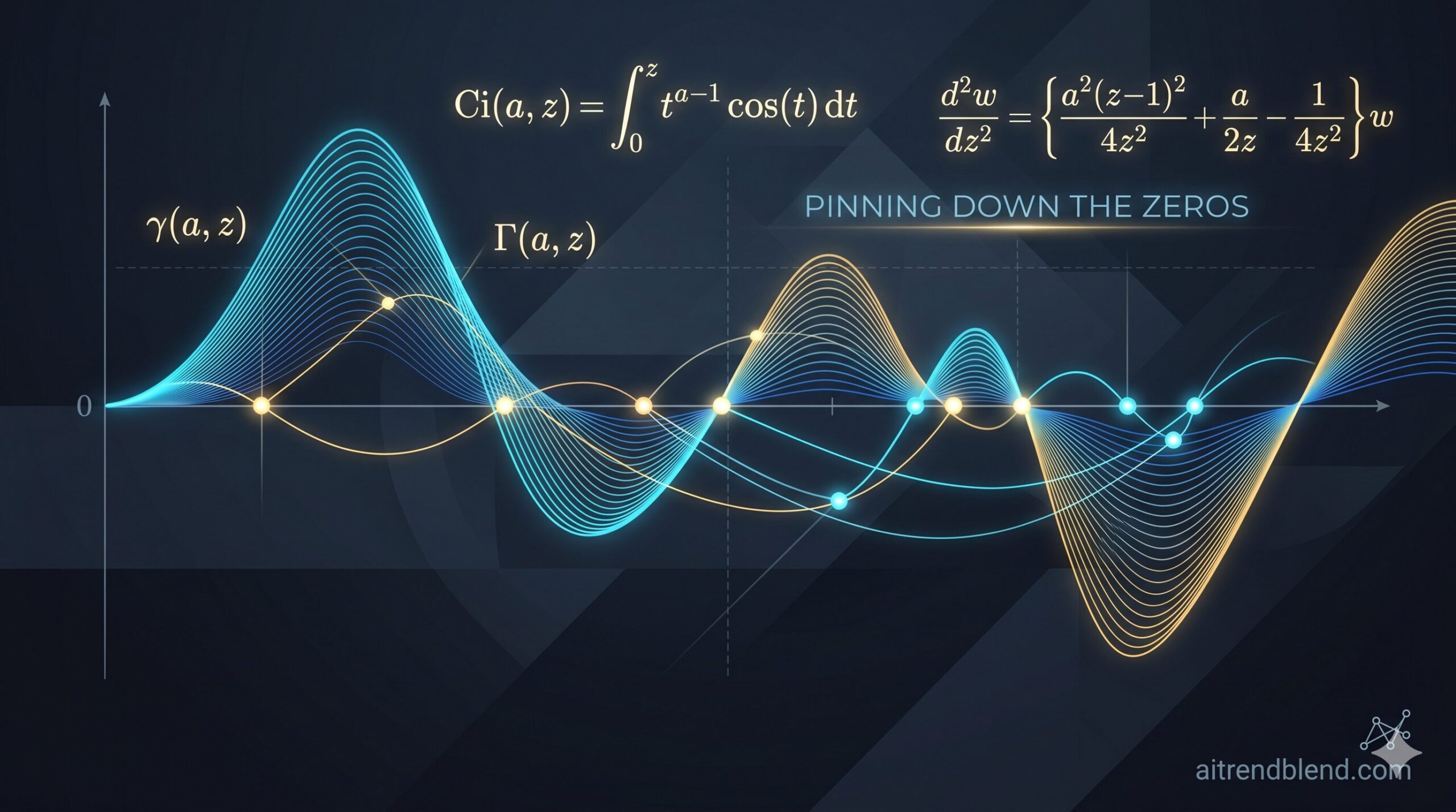
Generalised Trigonometric Integrals Asymptotic Expansions Zeros on the Real Line Liouville-Green Theory Incomplete Gamma Functions WKB Theory Special Functions Saddle Point Method

Imagine you are tracking all the places where a certain special function — built from an integral of a cosine or sine multiplied by a power — crosses zero on the real line. There are infinitely many of them, some clustered near the origin, others spreading out toward infinity. Now imagine finding a single formula that accurately locates every one of them, small or large, without needing a different approximation for each regime. That is exactly what T.M. Dunster has accomplished in this paper, and the technical machinery needed to get there is both deep and elegant.

What Are the Generalised Trigonometric Integrals, and Why Do They Matter?

The ordinary cosine integral $\mathrm{Ci}(z)$ and sine integral $\mathrm{si}(z)$ are workhorses of applied mathematics. They appear in antenna theory, diffraction optics, digital signal processing, and countless areas of physics and engineering where oscillating integrands with slowly decaying amplitudes come into play. Most science and engineering students encounter at least one of them during their training.

The generalised versions go one step further. Instead of just integrating $\cos(t)$ or $\sin(t)$ from zero to $z$, you weight the integrand by an additional factor $t^{a-1}$, where $a$ is a free real parameter. The four fundamental generalised trigonometric integrals (GTIs) are defined by:

The Four GTIs $$\mathrm{Ci}(a,z)=\int_0^z t^{a-1}\cos(t)\,dt,\quad \mathrm{Si}(a,z)=\int_0^z t^{a-1}\sin(t)\,dt$$ $$\mathrm{ci}(a,z)=\int_z^\infty t^{a-1}\cos(t)\,dt,\quad \mathrm{si}(a,z)=\int_z^\infty t^{a-1}\sin(t)\,dt$$

When $a=1$, you recover the classical integrals. For general $a$, these functions have richer structure — they gain additional oscillations, their zeros shift and multiply, and their behaviour near both the origin and infinity becomes substantially more complicated. The parameter $a$ acts almost like a dial that controls how rapidly the integrand’s power factor rises or falls relative to the oscillation rate.

Understanding where these functions vanish — their real zeros — is important in practice. Zero locations determine nodal patterns in wave problems, control stability of certain integral transforms, and arise in problems of signal reconstruction. Getting accurate approximations for all zeros simultaneously, not just the large ones, is both practically useful and mathematically non-trivial.

The Core Challenge in Plain Language

Classical asymptotic methods can tell you where the zeros are when they are very large — you just balance the dominant terms and expand. But the smallest zeros, close to the origin, behave very differently from the large ones, and stitching two separate approximations together is both messy and error-prone. Dunster’s paper delivers one unified formula that works for all zeros, small and large alike.

The Bridge Between Two Worlds — Incomplete Gamma Functions

The key insight in this paper is a connection that turns out to be a powerful shortcut: the generalised trigonometric integrals are not independent objects — they can be expressed directly in terms of the incomplete gamma functions. Specifically, $\mathrm{Ci}(a,z)$ and $\mathrm{Si}(a,z)$ are certain complex linear combinations of the lower incomplete gamma function $\gamma(a,z)$, and $\mathrm{ci}(a,z)$ and $\mathrm{si}(a,z)$ are analogous combinations of the upper incomplete gamma function $\Gamma(a,z)$:

GTIs via Incomplete Gamma Functions $$\mathrm{Ci}(a,z) = \tfrac{1}{2}e^{a\pi i/2}\gamma\!\left(a,ze^{-\pi i/2}\right) + \tfrac{1}{2}e^{-a\pi i/2}\gamma\!\left(a,ze^{\pi i/2}\right)$$ $$\mathrm{ci}(a,z) = \tfrac{1}{2}e^{a\pi i/2}\Gamma\!\left(a,ze^{-\pi i/2}\right) + \tfrac{1}{2}e^{-a\pi i/2}\Gamma\!\left(a,ze^{\pi i/2}\right)$$

This connection matters enormously, because the incomplete gamma functions are much better studied objects. The differential equation they satisfy is of a standard Liouville-Green (LG) type — the same kind of equation that underlies WKB theory in quantum mechanics and turning-point analysis in classical asymptotics. Once Dunster has uniform LG expansions for the incomplete gamma functions, the GTI expansions follow almost immediately by substitution.

The strategy, in broad strokes, is therefore: first build the asymptotic scaffolding for the incomplete gamma functions using LG theory, then transfer that scaffolding to the GTIs through the explicit connection formulas above, and finally exploit the resulting simple structure to locate zeros with high precision.

The Liouville-Green Engine — Turning a Differential Equation Into Asymptotics

The incomplete gamma functions $\gamma(a,az)$ and $\Gamma(a,az)$ — with the argument scaled to $az$ to make the large-$a$ structure transparent — satisfy a second-order linear differential equation of the form

The Governing ODE $$\frac{d^2w}{dz^2} = \left\{\frac{a^2(z-1)^2}{4z^2} + \frac{a}{2z} – \frac{1}{4z^2}\right\}w.$$

This is the entry point for Liouville-Green theory. The equation has a large parameter $a$ multiplying its leading term, which is exactly the setting where LG asymptotics shine. After a standard Liouville transformation — a change of both the independent variable and the dependent variable designed to put the equation into a simpler canonical form — one arrives at an equation whose solutions admit formal exponential asymptotic series in descending powers of $a$.

The crucial technical step is computing the LG expansion coefficients $E_s^-(z)$ explicitly. These are defined by successive integrations and recurrences, and for this particular equation they turn out to be rational functions of $z$ — a very clean and computationally friendly outcome. The first several are given in closed form:

First LG Coefficients (Explicit) $$E_0^-(z) = -\tfrac{1}{2}\ln(1-z),\quad E_1^-(z) = \frac{z}{(z-1)^2},\quad E_2^-(z) = \frac{z(3z+2)}{2(z-1)^4}$$

Being rational functions, each $E_s^-$ is easy to evaluate numerically, easy to differentiate symbolically, and easy to show is bounded at infinity. The paper proves, using a matching argument, that each coefficient approaches zero as $z \to \infty$ — a fact that turns out to be important when handling the upper incomplete gamma function, whose expansion is only valid away from the origin.

Two distinct LG solutions are constructed, one that is recessive (decaying) as $z \to 0$ and another that is recessive as $z \to +\infty$. The first matches the lower incomplete gamma function $\gamma(a,az)$; the second matches the upper incomplete gamma function $\Gamma(a,az)$. Their domains of asymptotic validity are described carefully using level curves of the Liouville phase function $\xi(z) = \tfrac{1}{2}(z-1) – \tfrac{1}{2}\ln z$, which has a saddle-point structure at $z=1$.

Why Two Solutions Are Needed

A single LG expansion cannot be uniformly valid everywhere: the solution recessive at zero grows at infinity, and vice versa. By constructing both and carefully tracking where each is valid, Dunster covers the entire real axis for the GTIs — the expansion for $\gamma$ is valid on the whole imaginary $z$-axis, while the expansion for $\Gamma$ is restricted to a half-plane away from the origin. This asymmetry turns out to be the source of some of the subtlety in the zero analysis.

From Gamma Functions to Trigonometric Integrals — The Explicit Expansions

With the incomplete gamma function expansions in hand, the GTI expansions follow by direct substitution into the connection formulas. For real argument $z = a\theta$ with $\theta > 0$, the results take a beautifully structured cosine-and-sine form. For example:

GTI Uniform Asymptotic Expansions $$\mathrm{Ci}(a,a\theta) = \frac{(a\theta)^a \exp\{\mathcal{E}_R(a,\theta)\}}{a\sqrt{\theta^2+1}}\cos\!\left(a\theta – \arctan\theta + \mathcal{E}_I(a,\theta)\right)$$ $$\mathrm{Si}(a,a\theta) = \frac{(a\theta)^a \exp\{\mathcal{E}_R(a,\theta)\}}{a\sqrt{\theta^2+1}}\sin\!\left(a\theta – \arctan\theta + \mathcal{E}_I(a,\theta)\right)$$

Here, $\mathcal{E}_R$ and $\mathcal{E}_I$ are the real and imaginary parts of the sum $\sum_{s=1}^\infty (-1)^s E_s^-(-i\theta)/a^s$, evaluated at purely imaginary argument $z = -i\theta$. These are real-valued asymptotic series in inverse powers of $a$, with coefficients computable from the explicit $E_s^-$ formulas above.

What makes this expansion remarkable is what it controls: the factor in front is a smoothly varying amplitude, while the oscillation is entirely captured by the cosine or sine term. The zeros of $\mathrm{Ci}(a,a\theta)$ occur precisely when the cosine vanishes — that is, when its argument equals a half-integer multiple of $\pi$. This transforms the zero-finding problem into an equation of the form

Zero Condition for Ci(a,aθ) $$a\,c_m – \arctan(c_m) + \mathcal{E}_I(a,c_m) = \left(m – \tfrac{1}{2}\right)\pi,\quad m = 1,2,3,\ldots$$

and the expansion structure allows this implicit equation to be solved systematically, yielding explicit formulas for every coefficient in the asymptotic expansion of each zero.

The Zero Expansion — A Recursive, Unified Formula for All Zeros

The main practical output of the paper is the uniform asymptotic expansion for the zeros themselves. Each zero $c_m$ of $\mathrm{Ci}(a,a\theta)$ admits the expansion

Zero Asymptotic Expansion $$c_m \sim c_{m,0} + \sum_{k=2}^{\infty}\frac{c_{m,k}}{a^k}\quad(a\to\infty,\; m=1,2,3,\ldots)$$

where the leading term $c_{m,0}$ is the root of the implicit equation

$a\,c_{m,0} – \arctan(c_{m,0}) = (m – \tfrac{1}{2})\pi.$

The higher-order correction terms $c_{m,k}$ are then given explicitly by $c_{m,k} = q_k(c_{m,0})$, where $q_k(x)$ are universal rational functions of $x$ — independent of both $m$ and $a$. The same functions $q_k$ appear for all zeros. The first two non-trivial corrections are:

First Correction Terms $$q_2(x) = \frac{x(x^2-1)}{(x^2+1)^2},\qquad q_3(x) = \frac{4x^3(2x^2-3)}{(x^2+1)^4}$$

These rational functions vanish at both $x=0$ and $x=\infty$, which confirms that the corrections are negligible at both extremes of the zero distribution — the expansion is uniformly valid from the smallest zero to arbitrarily large ones. Including ten correction terms in the approximation (the paper checks this numerically for $a = 10$ and $a = 20.5$) gives results accurate to many decimal places simultaneously for all one hundred zeros tested.

“The coefficients in the zero asymptotic expansions are recursively defined rational functions of the first coefficient in the expansion for each zero, which itself can be readily computed as a root of an implicit equation.” — T.M. Dunster · J. Math. Anal. Appl. 560 (2026)

The same structure repeats for the zeros of $\mathrm{Si}(a,a\theta)$ and for the linear combination $\mathrm{Ti}(a,a\theta,\alpha)$ — in each case the leading term satisfies a slightly different implicit equation, but the correction rational functions $q_k(x)$ are exactly the same. This universality is a sign of the deep structural unity underlying the whole family of GTIs.

The Harder Case — Zeros of the Complementary Functions ci and si

The complementary integrals $\mathrm{ci}(a,z)$ and $\mathrm{si}(a,z)$ — defined as integrals from $z$ to infinity — are harder to handle. Here is why: the LG expansion for the upper incomplete gamma function $\Gamma(a,az)$ is not valid on the entire imaginary axis in $z$, unlike the lower incomplete gamma function expansion. So Dunster cannot directly substitute $z = -i\theta$ in the same clean way.

Instead, he derives an equation for the zeros of $\mathrm{ci}(a,a\theta)$ that involves a comparison with the zeros of $\mathrm{Ci}(a,a\theta)$. The key observation is that for large $a$, the function

The Modulation Function χ $$\chi(a,\theta) = \frac{\Gamma(a+1)\cos\!\left(\tfrac{1}{2}\pi a\right)\sqrt{\theta^2+1}}{(a\theta)^a}$$

decays extremely rapidly as $\theta$ increases, because of the Stirling-type growth of $(a\theta)^a$ in the denominator. This means that for all but the very first few zeros, $\chi$ is negligible, and the zeros of $\mathrm{ci}$ are exponentially close to those of $-\mathrm{Ci}$. Only the smallest zeros — those close to the transition region where $|\chi| \approx 1$ — genuinely differ from the pattern.

Large Zeros of ci(a,aθ)

When $\tilde{c}_{m,0}$ is sufficiently large, $|\chi(a,\tilde{c}_{m,0})| \to 0$ rapidly. The correction terms $\tilde{q}_k$ then reduce exactly to the same rational functions $q_k$ already derived for $\mathrm{Ci}$, confirming consistency between the two families of zeros far from the origin.

Transition Zeros — The Delicate Case

Near the transition point where $|\chi| \approx 1$, the expansion coefficients $\tilde{q}_k$ have denominators that can approach zero. The paper handles this carefully with a dedicated lemma showing that at most one zero can ever sit in this delicate region — so the singular case is genuinely isolated, not systemic.

The correction rational functions $\tilde{q}_k(x)$ for the $\mathrm{ci}$ zeros are analogues of $q_k$ but now carry the quantities $C = \chi(a,\tilde{c}_{m,0})$ and $S = \sqrt{1-C^2}$ as parameters. For example:

First Correction for ci Zeros $$\tilde{q}_2(x) = \frac{x^2\!\left(Sx^2 + 2Cx – S\right)}{(x^2+1)^2(Sx – C)}$$

When $C = 0$ and $S = 1$, this collapses exactly to $q_2(x)$, as it must. The transition parameter $C$ smoothly interpolates between the $\mathrm{ci}$ regime and the $\mathrm{Ci}$ regime as the zeros grow larger.

The Key Lemma — At Most One Problematic Zero

One of the most technically satisfying results in the paper is Lemma 3.1, which resolves the potentially awkward situation where the denominator $Sx – C$ appearing in the correction formulas could vanish. If that happened for many zeros simultaneously, the whole expansion would be in trouble. But the lemma rules this out definitively:

Lemma 3.1 — The Isolation Principle

For each value of $a$ satisfying $|\cos(\tfrac{1}{2}\pi a)| \geq \delta > 0$, there is at most one index $m$ for which the leading approximation $\tilde{c}_{m,0}$ satisfies $Sx – C = o(1)$ as $a \to \infty$.

All other zeros in the sequence have their denominators bounded away from zero, so the asymptotic expansion for those zeros is uniformly valid without any special treatment.

The proof is elegant: it shows that the problematic transition occurs near $\tilde{c}_{m,0} \approx e^{-1}$, and then uses the fact that consecutive leading terms $\tilde{c}_{m,0}$ and $\tilde{c}_{m+1,0}$ are spaced at least a fixed positive distance apart (of order $1/a$), combined with the exponential decay of $\chi$, to confirm that once one zero passes through the transition, all subsequent ones are safely in the regime where $C$ is negligible.

For that one exceptional zero — if it exists for a particular $a$ — the paper provides a fallback: set $\theta = \tilde{c}_{m,0} + \epsilon$ in the zero equation and solve numerically for the small correction $\epsilon$. This is always computable, just not in closed asymptotic form.

Numerical Verification — How Good Is Ten Terms?

The paper does not merely state the expansions — it checks them quantitatively. Using a relative error measure $\Delta(a,\theta)$ defined in terms of the ratio of the function value to its derivative at the approximate zero, the accuracy of the ten-term expansion is visualised by plotting $\log_{10}|\Delta(a,\theta_{m,10}(a))|$ for $m = 1, 2, \ldots, 100$.

The results are impressive. At $a = 10$, ten correction terms deliver approximately eight to ten decimal digits of accuracy for every zero in the first one hundred. At $a = 20.5$, the accuracy improves further — in the range of ten to fourteen decimal digits for most zeros. The uniformity across all one hundred zeros, from the very smallest to the hundredth, confirms that this is genuinely a uniform expansion in the classical sense: no special treatment is needed for small zeros, and no accuracy is lost at large ones.

Why Uniformity Is Significant

A non-uniform expansion might give fifteen digits of accuracy for the hundredth zero and only two for the first. A uniform expansion, by contrast, provides comparable accuracy across the board. This matters enormously in practice: you can trust the formula for any zero without first checking whether that zero is in a “good” or “bad” regime. Dunster’s expansions achieve exactly this kind of blanket reliability.

Applications and the Broader Context

The generalised trigonometric integrals arise across a wide range of applied problems. In electromagnetic theory, the classical cosine and sine integrals appear in antenna radiation patterns and the evaluation of field integrals. In optics, they describe diffraction by straight edges and slit apertures. In digital signal processing, they model the frequency response of certain filtering operations. The generalised versions with free parameter $a$ are relevant whenever the physical problem involves an additional power-law weighting — for instance, in problems with tapered or weighted apertures.

Getting accurate zero locations for these functions matters because the zeros often correspond to physically significant features: the dark fringes in a diffraction pattern, the nulls in an antenna beam, or the nodal frequencies of a filtered signal. Previous work, notably by Nemes (2025) and Temme (1995), had addressed related questions for either the zeros of the incomplete gamma functions or for the large-argument asymptotics of GTIs with computable error bounds. Dunster’s paper extends both lines of work by providing the first truly uniform expansion covering all zeros simultaneously for large $a$.

The method itself — building LG expansions for a governing differential equation, matching them to known special functions, and then differentiating the structure to extract zero asymptotics — is a template that can be applied to many other families of integrals and orthogonal polynomials. The explicit error bound framework, derived from general LG theory (Dunster, 2020), makes the approach not just formal but rigorous and computable, which is increasingly important as numerics and asymptotics become more tightly integrated in computational mathematics.

What the Paper Leaves Open — and Where This Line of Work Goes Next

A few natural extensions remain open. The paper focuses on real zeros with real positive $\theta$; a complete treatment of complex zeros would require extending the LG domains into the complex $z$-plane more aggressively, which the author notes is possible but not pursued here. Similarly, the behaviour of the zeros at the transition between the $\mathrm{Ci}$ and $\mathrm{ci}$ regimes — handled by the isolation lemma for that one exceptional index — could in principle be developed into a uniform transition expansion in its own right, analogous to Airy-function transition asymptotics for turning-point problems.

There is also the question of what happens when $a$ is complex or in certain other parameter regimes. The LG theory used here is valid for real positive $a$, but modern LG methods extend to sectors in the complex plane, suggesting that the zero analysis could eventually be extended to complex parameter values as well.

From a broader perspective, papers like this one sit at the fertile intersection of classical analysis and modern computation. The explicit rational functions $q_k(x)$ for the zero corrections are immediately useful in software libraries for special functions — a user implementing a fast evaluator for GTI zeros can simply tabulate these rational functions once and then apply the expansion at negligible computational cost for any $m$ and $a$. The combination of mathematical rigour, explicit formulas, and numerical verification makes the result directly deployable, not merely theoretically satisfying.

Read the Full Paper

Published open access in the Journal of Mathematical Analysis and Applications, Volume 560 (2026), under the CC BY license. Full proofs, error bound theorems, and numerical verification figures are available via the journal’s website.

📄 Read the Paper (DOI) 🔗 JMAA Journal Page

Academic Citation:
T.M. Dunster. Uniform asymptotic expansions for generalised trigonometric integrals and their zeros. Journal of Mathematical Analysis and Applications, 560 (2026) 130493. https://doi.org/10.1016/j.jmaa.2026.130493

This article is an independent editorial analysis of a peer-reviewed open-access paper published under the CC BY 4.0 license. Mathematical statements paraphrase the original results; for complete proofs, error bounds, and precise formulations, consult the published paper. The paper was received August 11, 2025, and made available online February 6, 2026.

References

[1] L. Comtet. Advanced Combinatorics: The Art of Finite and Infinite Expansions. Springer, Dordrecht, 1974.
[2] T.M. Dunster. Asymptotic solutions of second-order linear differential equations having almost coalescent turning points, with an application to the incomplete gamma function. Proc. R. Soc. Lond. A 452 (1996) 1331–1349.
[3] T.M. Dunster. Liouville-Green expansions of exponential form, with an application to modified Bessel functions. Proc. R. Soc. Edinb., Sect. A, Math. 150 (2020) 1289–1311.
[4] T.M. Dunster. Uniform asymptotic expansions for the zeros of Bessel functions. SIAM J. Math. Anal. 56 (2024) 6521–6550.
[5] T.M. Dunster. Uniform asymptotic expansions for Bessel functions of imaginary order and their zeros. Integral Transforms Spec. Funct. (2025) 1–32.
[6] K. Iizuka. Engineering Optics, 3rd ed. Springer, New York, 2008.
[7] N. Lebedev. Special Functions and Their Applications. Prentice-Hall, Englewood Cliffs, New Jersey, 1965.
[8] D. Manolakis, V. Ingle. Applied Digital Signal Processing: Theory and Practice. Cambridge University Press, Cambridge, 2011.
[9] G. Nemes. Asymptotic expansions for the generalised trigonometric integral and its zeros. J. Math. Anal. Appl. 549 (2025).
[10] NIST Digital Library of Mathematical Functions, Release 1.1.6 of 2022-06-30, http://dlmf.nist.gov/, F.W.J. Olver et al. (Eds.).
[11] F.W.J. Olver. Asymptotics and Special Functions. A K Peters Ltd., Wellesley, MA, 1997.
[12] N.M. Temme. The asymptotic expansion of the incomplete gamma functions. SIAM J. Math. Anal. 10 (1979) 757–766.
[13] N.M. Temme. Asymptotics of zeros of incomplete gamma functions. Ann. Numer. Math. 2 (1995) 415–423.