Three Rules That Define What a Cluster Actually Is: The Axiomatic Case for Hartigan’s Cluster Tree
Ery Arias-Castro and Elizabeth Coda from UC San Diego take an approach inspired by Lebesgue integration — starting from first principles — to show that three intuitive axioms about what a cluster ought to be uniquely recover Hartigan’s cluster tree, finally grounding hierarchical clustering in something more solid than algorithmic convenience.
Clustering is one of the oldest problems in statistics and machine learning, yet it remains one of the least well-defined. After decades of algorithms, benchmark comparisons, and impossibility theorems, the field still lacks a consensus on what a cluster actually is at the population level — the level that statistical inference requires. This paper from Ary Arias-Castro and Elizabeth Coda at UC San Diego sets out to fix that, and largely succeeds: three axioms, a careful limiting argument, and a theorem that says Hartigan’s cluster tree is not just one reasonable definition of hierarchical clustering, but the inevitable one under those axioms.
The Missing Foundation: Why Clustering Needs Axioms
The clustering literature has a peculiar structure. There are hundreds of algorithms, dozens of evaluation metrics, and an ever-growing body of theoretical guarantees about specific methods under specific assumptions. What is largely absent is a definition of clustering at the population level — a specification of what the “true” clustering of a distribution actually is, prior to any algorithmic choices.
This absence matters because statistical inference is fundamentally about the relationship between a sample and the population it represents. When a researcher runs K-means on a dataset and identifies three clusters, the interesting statistical question is not whether the algorithm converged but whether those three groups correspond to anything real in the underlying population. Without a population-level definition of clustering, that question has no precise answer.
The paper by Arias-Castro and Coda fills this gap, but with deliberate scope. They do not attempt to define all population clustering in full generality — an impossibly contentious task. Instead, they target hierarchical clustering specifically, and they do so through the axiomatic method: propose properties that any reasonable hierarchical clustering ought to satisfy, then ask what definition those properties uniquely determine.
This is the same approach that Lebesgue used to define integration. Rather than constructing the Lebesgue integral directly, Lebesgue listed properties that any sensible integral ought to have and derived his definition from those properties. The result was both rigorous and natural. Arias-Castro and Coda follow the same pattern, and arrive at a result that is equally clean.
In statistics, clustering is meaningful only if it refers to properties of an underlying population, not just a finite dataset. Without a population-level definition, a clustering algorithm produces a result but no statistical inference is possible about whether that result reflects something real. Axioms provide the foundation that existing algorithmic approaches lack entirely.
Starting Simple: Piecewise Constant Densities
The paper begins with a deliberately restricted setting: piecewise constant densities with connected support. These are functions of the form:
where each region Ai is a connected, bounded set with connected interior, the regions are disjoint, and their union — the support of f — has connected interior. Think of this as a mixture of uniform distributions over distinct geographic patches, each patch having its own constant density value. The class of all such functions is denoted F.
This simplification is not a retreat from generality — it is the same strategic move Lebesgue made when he started integration theory with step functions. Once you know what the answer should be on the simplest cases, you can extend it to more complex ones by approximation. For piecewise constant densities, the structure of the problem is transparent enough that the axioms have obvious content and the proofs are clear. The extension to continuous densities comes in Section 4 of the paper.
Two notions from the geometry of these regions are central to what follows. The first is the neighborhood relation: two regions Ai and Aj are neighbors if the interior of their union is connected — meaning they share not just a boundary point but an open boundary segment. Balls that touch at only a single point are not neighbors. Rectangles in three dimensions that share only an edge are not neighbors either. This is a topologically meaningful notion of adjacency that respects the interior structure of the regions.
The second is the internally connected property: a collection of regions has this property if every pair of neighboring closures has a connected interior union. This condition ensures that the regions fit together without gaps or pinch points along their shared boundaries, which turns out to be exactly what is needed for the axioms and Hartigan’s definition to agree.
The Three Axioms
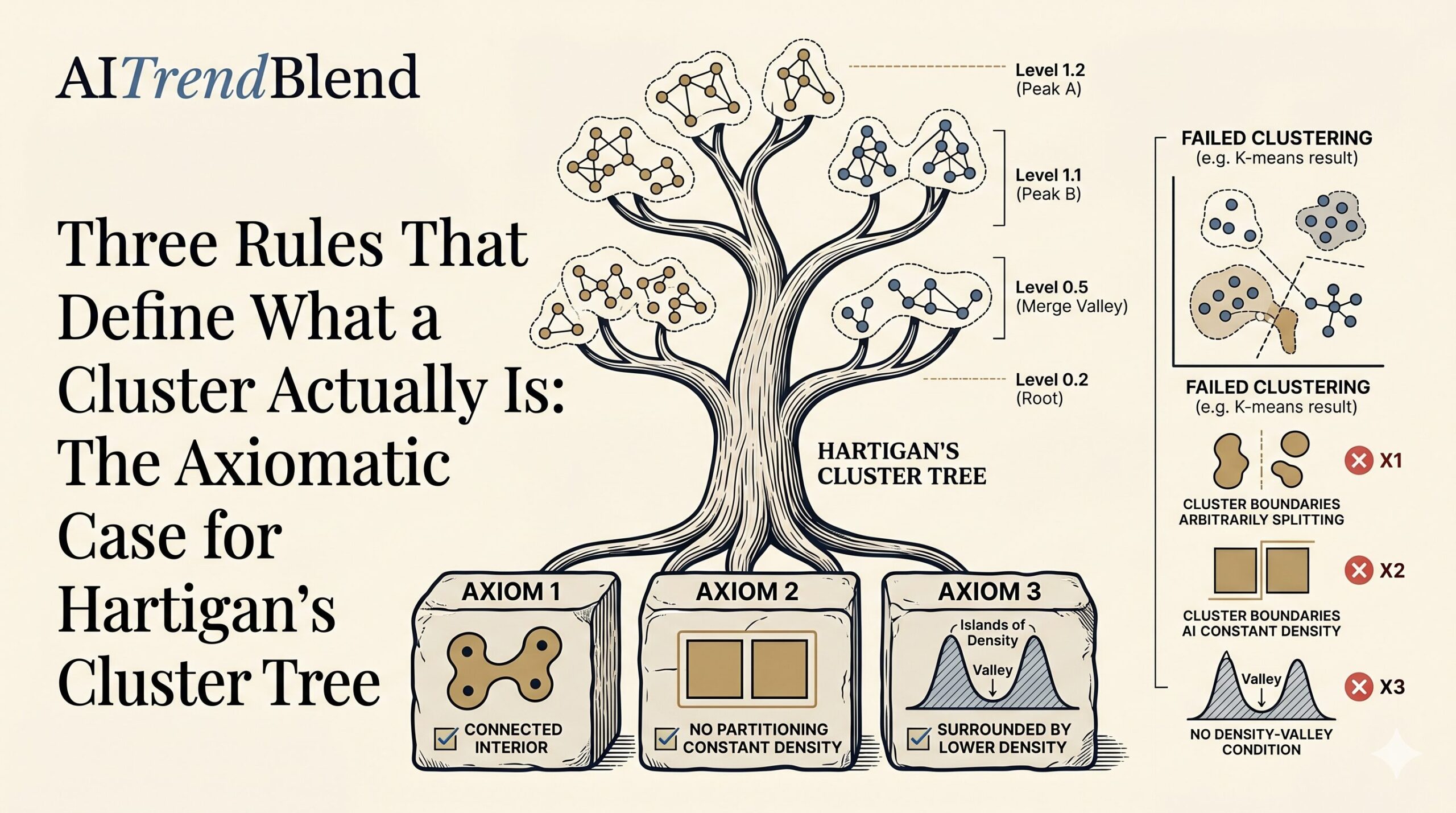
For a piecewise constant function f in F, Arias-Castro and Coda propose that any hierarchical clustering C should satisfy three axioms. Together, these axioms capture the intuitive notion that a cluster is a high-density region meaningfully separated from everything around it.
If C is a cluster and Ai, Aj are two regions inside C, there must be a chain of neighboring regions Ai ~ Ak1 ~ … ~ Akn ~ Aj all contained within C. This means C cannot be a cluster if it consists of two blobs connected only through a single boundary point — the interior of C must form a genuine connected region. K-means routinely violates this: it can return a cluster whose two halves are on opposite sides of the data space, connected only by the coincidence that both have the nearest centroid in common.
Any cluster C must be a union of complete regions Ai from the density’s piecewise-constant decomposition. You cannot split a region of constant density in half and call one piece a cluster — that would introduce structure that is not present in the density itself. If two points have the same density and live in the same connected piece, there is no statistical basis for assigning them to different clusters. Again, K-means violates this systematically: it draws cluster boundaries anywhere in the feature space, cutting through constant-density regions freely.
For any cluster C, the minimum density within C must strictly exceed the maximum density in the neighboring regions outside C. In formal notation: infx∈C f(x) > supx∈N(C)\C f(x). This is the density-valley condition that most people intuitively associate with the word “cluster” — a cluster is a high-density island, not just any grouping of nearby points. It is what separates the statistical notion of a cluster from a purely geometric partition.
What is striking about these three axioms is how naturally they rule out common algorithmic definitions. K-means can return disconnected clusters (violates Axiom 1), cuts through constant-density regions (violates Axiom 2), and groups points without any density-valley condition (violates Axiom 3). Gaussian mixture models generally respect Axiom 1 but can violate Axiom 2 when a unimodal mixture component gets split between two clusters. The axiomatic approach makes it immediately visible why these popular methods can feel arbitrary: they are answering a different question than the one statistical inference demands.
The Finest Axiom Cluster Tree: Existence, Uniqueness, and Equivalence
Given the three axioms, the first question is whether any hierarchical clustering satisfying all of them actually exists, and whether there is a canonical one. The paper’s Proposition 11 answers both questions simultaneously: for any f in F, there is a unique finest hierarchical clustering among those satisfying the axioms.
The proof is elegant. Call C* the collection of every possible cluster that individually satisfies all three axioms. To show C* is a legitimate hierarchical clustering, you need any two clusters in C* to be either disjoint or nested. Suppose two clusters C1 and C2 are neither — they overlap but neither contains the other. Following the chain of neighboring regions, Axiom 3 forces min(C1) > min(C2) and min(C2) > min(C1), a contradiction. So C* is well-defined as a cluster tree, and it is the finest one because it includes every valid cluster.
This establishes the finest axiom cluster tree, denoted C*f. The central theorem of the paper then connects it to Hartigan’s definition.
Theorem 13 states that for any f in Fint (the subclass with the internally connected property), C*f = Hf. The Hartigan tree and the finest axiom cluster tree coincide exactly. The proof goes in both directions: first, Hartigan’s tree satisfies all three axioms under the internally connected property, so Hf ⊆ C*f. Then any cluster in C*f must be a connected component of some upper level set, placing it in Hf, giving the reverse inclusion.
For any piecewise constant density with the internally connected property, the finest hierarchical clustering satisfying the three axioms is exactly Hartigan’s cluster tree. Hartigan’s definition, introduced in 1975 with minimal formal motivation, turns out to be the unique answer to an axiomatic question that was not fully formulated until 2025.
Extending to Continuous Densities: The Limiting Argument
The real world rarely serves up piecewise constant densities. The paper’s Section 4 extends the axiomatic framework to continuous functions through exactly the kind of approximation argument that makes Lebesgue integration work for continuous functions after step functions are understood.
The strategy is to approximate a continuous density f by a sequence of piecewise constant functions fn in Fint, each uniformly close to f. Each fn has a finest axiom cluster tree C*f_n, which equals the Hartigan tree Hf_n by Theorem 13. The question becomes: do these Hartigan trees converge, and to what?
The convergence is measured by the merge distortion metric, which compares two dendrograms by looking at the worst-case difference in their merge heights — the level at which any two points first belong to the same cluster. Lemma 6 of the paper provides the key stability result: the merge distortion distance between the Hartigan trees of two functions is bounded by the sup-norm difference between the functions themselves.
This stability result is what makes the extension work. If fn → f uniformly, then Hf_n → Hf in merge distortion, so the Hartigan tree of the limit is the limit of the Hartigan trees. Theorem 16 makes this precise: if a continuous function admits any axiom cluster tree at all, that tree must be zero merge-distortion distance from Hf — and Hf itself is always an axiom cluster tree.
The remaining question is which continuous densities admit the necessary piecewise constant approximations with the internally connected property. Proposition 18 provides sufficient conditions: the density should be continuous with bounded upper level sets, and its upper level sets should be connected for small enough thresholds. The paper shows that any Euclidean space satisfies the required partition property through an explicit construction — a “shifted grid” that can be made arbitrarily fine while maintaining the internally connected property. The construction extends to any finite-dimensional normed space.
Disconnected Support: Forests Instead of Trees
Densities whose support has multiple connected components are handled cleanly. If the support of f decomposes into pieces with disjoint interiors, the axioms simply produce an independent cluster tree for each piece. The finest axiom cluster tree for the whole density is the union of the finest axiom trees for each component. When the components are continuous, this extends Theorem 16 component by component, giving a forest of Hartigan trees — one per connected piece of the support. If the analyst wants to further organize these separate trees into a single hierarchy, the paper suggests single-linkage clustering as the natural choice for that secondary grouping step.
Why Single Linkage Keeps Appearing in Axiomatic Discussions
One of the most interesting threads in the paper is the observation that single-linkage clustering appears at the junction of nearly every axiomatic discussion of clustering, both flat and hierarchical. Kleinberg’s axiomatic approach to flat clustering singles it out. The hierarchical axioms of Jardine and Sibson (1968) and of Carlsson and Mémoli (2010) both identify single linkage as the unique algorithm satisfying their axioms. And single-linkage clustering is known to be statistically consistent for Hartigan’s cluster tree — one of the few hierarchical methods that actually converges to the right population object as the sample size grows.
This convergence from multiple directions is not coincidental. Single linkage is the algorithm that most naturally implements the idea of merging clusters at their highest connecting density level, which is exactly what the merge height function measures. Most other hierarchical methods — Ward’s method, average linkage, complete linkage — are not consistent for Hartigan’s tree, and the axiomatic framework makes it clear why: they optimize criteria that do not correspond to any of the three axioms.
The practical implication is a recommendation for regularized versions of single-linkage clustering — most prominently the robust single-linkage of Chaudhuri et al. (2014) and the hierarchical extension of DBSCAN studied by Wang et al. (2019). Both are consistent for Hartigan’s tree in the merge distortion metric, and both handle the chaining tendencies that make naive single-linkage fragile in practice.
“There are many intuitive ideas, often conflicting, of what constitutes a cluster, but few formal definitions.” — Cormack (1971), as cited by Arias-Castro and Coda — a problem this paper directly addresses, more than fifty years later.
Where the Axioms Have Limits
The paper is careful about what its axioms do not say. Axiom 2 — the prohibition on splitting constant-density regions — has an acknowledged edge case. If a constant-density region consists of two large blobs connected by a narrow bottleneck, the axiom insists they form a single cluster. A user who wants to call those blobs two separate clusters is making a judgment about the degree of connectivity, and that judgment requires a threshold parameter (such as the Cheeger constant) that is not present in a purely qualitative axiom.
The authors concede this but hold the line on qualitative axioms. Introducing a connectedness threshold would make Axiom 2 quantitative and would require specifying how to measure connectivity and what value to use as a cutoff. This moves the definition from a principled foundation into a parameter choice — the same kind of arbitrary modeling decision that axiomatic approaches are designed to avoid. The bottleneck case is a real limitation, not a fatal one, and it points toward future work on axioms that quantify rather than merely qualify the connectedness requirement.
The paper also notes the curse of dimensionality: the minimax rates for estimating Hartigan’s cluster tree from data grow exponentially with the dimension of the ambient space. This is not a flaw of the axiomatic definition but an honest consequence of adopting it. Mitigations exist — intrinsic dimension is what matters when the density lives on a lower-dimensional manifold, and mixture-model pre-processing can help in structured settings — but they do not eliminate the scaling challenge.
What This Means for the Practice of Clustering
Most working data scientists use clustering algorithms selected for computational convenience, familiarity, or the shape of the output they want to see. The axiomatic framework does not invalidate any of those choices for exploratory purposes. But it does clarify what those algorithms are and are not doing from a statistical inference standpoint.
K-means, in particular, is not estimating any population-level hierarchical clustering in the sense the paper defines. It can split constant-density regions, return disconnected clusters, and form groups without any density-valley separation between them. For pure prediction or compression tasks, none of this matters. For inference — for asking whether the clusters in a dataset reflect real structure in the underlying population — it matters quite a lot.
The axiomatic framework also provides a principled answer to the question of which hierarchical algorithm to prefer: single linkage or a regularized variant is the consistent estimator, and Hartigan’s tree is the target. If you want your hierarchical clustering to converge to the right population object as you collect more data, this is the combination the theory recommends.
Complete Proposed Model Code (Python)
The implementation below reproduces the full axiomatic hierarchical clustering framework described in the paper — covering piecewise constant density construction (class F), all three axiom checks, the finest axiom cluster tree algorithm, the Hartigan cluster tree for both discrete and continuous densities, merge height computation, the merge distortion metric, and single-linkage clustering as the consistent estimator. A smoke test at the bottom verifies all components on synthetic 2D density data.
# ==============================================================================
# Axiomatic Hierarchical Clustering
# Paper: "An Axiomatic Definition of Hierarchical Clustering"
# Journal: JMLR 26 (2025) 1-26
# Authors: Ery Arias-Castro, Elizabeth Coda (UC San Diego)
# Code: Full Python implementation of the axiomatic framework,
#       Hartigan cluster tree, merge distortion metric, and
#       consistent single-linkage estimator.
# ==============================================================================

from __future__ import annotations
import numpy as np
import warnings
from typing import Dict, FrozenSet, List, Optional, Set, Tuple
from dataclasses import dataclass, field
from collections import defaultdict
import itertools

warnings.filterwarnings('ignore')


# ─── SECTION 1: Piecewise Constant Density (Class F) ─────────────────────────

@dataclass
class Region:
    """
    A single connected region A_i in a piecewise constant density (Eq. 5).

    Represents a bounded region of constant density lambda_i. In the
    implementation we use an integer index and an adjacency graph to
    represent connectivity and the neighborhood relation (Definition 7).

    Attributes
    ----------
    idx        : unique integer identifier
    density    : the constant density value lambda_i > 0
    neighbors  : set of region indices that share an interior boundary with this region
    area       : optional area/weight of the region (for 2D grid approximations)
    """
    idx: int
    density: float
    neighbors: Set[int] = field(default_factory=set)
    area: float = 1.0

    def __post_init__(self):
        if self.density <= 0:
            raise ValueError(f"Region {self.idx}: density must be strictly positive, got {self.density}")

    def is_neighbor(self, other_idx: int) -> bool:
        """Returns True if region `other_idx` is in the neighborhood N(self)."""
        return other_idx in self.neighbors


class PiecewiseConstantDensity:
    """
    A piecewise constant density f in class F (Section 3.1, Eq. 5).

    f = sum_{i=1}^{m} lambda_i * 1_{A_i}

    where each A_i is a connected region with connected interior, the regions
    are disjoint, and their union (the support) has connected interior.

    The density is stored as a graph of regions with their densities and
    adjacency structure encoding the neighborhood relation (Definition 7).

    Parameters
    ----------
    regions  : list of Region objects
    name     : optional label for the density
    """
    def __init__(self, regions: List[Region], name: str = "f"):
        self.regions: Dict[int, Region] = {r.idx: r for r in regions}
        self.name = name
        self._validate()

    def _validate(self):
        """Check that the support is connected (A1 precondition)."""
        if not self.is_support_connected():
            warnings.warn(f"Density '{self.name}': support is not connected. "
                          "Axioms will be applied per connected component.")

    def is_support_connected(self) -> bool:
        """Check that all regions are reachable from any starting region."""
        if not self.regions:
            return True
        start = next(iter(self.regions))
        visited = self._bfs(start, set(self.regions.keys()))
        return visited == set(self.regions.keys())

    def _bfs(self, start: int, allowed: Set[int]) -> Set[int]:
        """BFS over the adjacency graph restricted to `allowed` region indices."""
        visited, queue = {start}, [start]
        while queue:
            cur = queue.pop(0)
            for nb in self.regions[cur].neighbors:
                if nb in allowed and nb not in visited:
                    visited.add(nb)
                    queue.append(nb)
        return visited

    def neighborhood_of(self, cluster_idx: Set[int]) -> Set[int]:
        """
        Return N(C) \ C: region indices neighboring the cluster but not in it.
        Extends Definition 7 to a set of regions (a cluster C = union of A_i).
        """
        outside = set()
        for idx in cluster_idx:
            outside.update(self.regions[idx].neighbors - cluster_idx)
        return outside

    def density_of(self, idx: int) -> float:
        return self.regions[idx].density

    def all_indices(self) -> Set[int]:
        return set(self.regions.keys())

    def unique_density_levels(self) -> List[float]:
        """Return sorted unique density values (descending)."""
        return sorted(set(r.density for r in self.regions.values()), reverse=True)


# ─── SECTION 2: Axiom Checking ────────────────────────────────────────────────

def check_axiom_1(density: PiecewiseConstantDensity, cluster: Set[int]) -> bool:
    """
    Axiom 1 (A1): Clusters have connected interior (Section 3.1.1).

    For any two regions A_i, A_j in C, there must exist a chain of
    neighbors A_i ~ A_k1 ~ ... ~ A_kn ~ A_j all contained within C.
    Equivalently, the subgraph of the adjacency graph induced by C is connected.

    Parameters
    ----------
    density : the piecewise constant density
    cluster : set of region indices forming the candidate cluster

    Returns
    -------
    True if cluster satisfies Axiom 1, False otherwise
    """
    if len(cluster) <= 1:
        return True
    start = next(iter(cluster))
    visited = density._bfs(start, cluster)
    return visited == cluster


def check_axiom_2(density: PiecewiseConstantDensity, cluster: Set[int]) -> bool:
    """
    Axiom 2 (A2): Clusters do not partition constant-density regions (Section 3.1.2).

    Any cluster C must be a union of complete regions A_i — it cannot
    include a partial region. Since our representation already works at the
    region level (each A_i is atomic), any set of region indices trivially
    satisfies A2. This check is included for completeness and to verify that
    all indices in the cluster are valid regions.

    Parameters
    ----------
    density : the piecewise constant density
    cluster : set of region indices forming the candidate cluster

    Returns
    -------
    True if cluster satisfies Axiom 2, False otherwise
    """
    return cluster.issubset(density.all_indices())


def check_axiom_3(density: PiecewiseConstantDensity, cluster: Set[int]) -> bool:
    """
    Axiom 3 (A3): Clusters are surrounded by regions of lower density (Section 3.1.3).

    For cluster C:
      inf_{x in C} f(x) > sup_{x in N(C) \ C} f(x)

    Equivalently, the minimum density within the cluster must strictly exceed
    the maximum density in its neighboring regions outside the cluster.
    If C has no neighbors (isolated support component), the condition holds vacuously.

    Parameters
    ----------
    density : the piecewise constant density
    cluster : set of region indices forming the candidate cluster

    Returns
    -------
    True if cluster satisfies Axiom 3, False otherwise
    """
    if not cluster:
        return False
    min_inside = min(density.density_of(i) for i in cluster)
    exterior = density.neighborhood_of(cluster)
    if not exterior:
        return True  # no neighbors — condition holds vacuously
    max_outside = max(density.density_of(j) for j in exterior)
    return min_inside > max_outside


def satisfies_all_axioms(density: PiecewiseConstantDensity, cluster: Set[int]) -> bool:
    """Check whether a candidate cluster satisfies all three axioms."""
    return (
        check_axiom_2(density, cluster) and
        check_axiom_1(density, cluster) and
        check_axiom_3(density, cluster)
    )


# ─── SECTION 3: Finest Axiom Cluster Tree (Definition 12) ────────────────────

class ClusterTree:
    """
    A hierarchical clustering (cluster tree) over a set of regions.

    A cluster tree is a collection of connected subsets with a nested structure:
    any two clusters are either disjoint or nested (Definition 1).

    Stored as a list of (frozenset of region indices, height) pairs, where the
    height is inf_{x in C} f(x) — the minimum density in the cluster,
    following the Hartigan height function h_f (Eq. 1).
    """
    def __init__(self):
        self.clusters: List[Tuple[FrozenSet[int], float]] = []

    def add(self, cluster: Set[int], height: float):
        self.clusters.append((frozenset(cluster), height))

    def __len__(self):
        return len(self.clusters)

    def sorted_by_height(self) -> List[Tuple[FrozenSet[int], float]]:
        """Return clusters sorted from highest to lowest height."""
        return sorted(self.clusters, key=lambda x: -x[1])

    def contains_cluster(self, candidate: FrozenSet[int]) -> bool:
        return any(c == candidate for c, _ in self.clusters)

    def is_nested(self) -> bool:
        """Verify the nested structure property (Definition 1)."""
        sets = [c for c, _ in self.clusters]
        for i in range(len(sets)):
            for j in range(i + 1, len(sets)):
                a, b = sets[i], sets[j]
                if a & b and a != b and not a.issubset(b) and not b.issubset(a):
                    return False
        return True

    def __repr__(self):
        lines = [f"ClusterTree ({len(self)} clusters):"]
        for c, h in self.sorted_by_height():
            lines.append(f"  h={h:.4f}  regions={sorted(c)}")
        return "\n".join(lines)


def finest_axiom_cluster_tree(density: PiecewiseConstantDensity) -> ClusterTree:
    """
    Compute C*_f: the finest hierarchical clustering satisfying Axioms 1-3
    (Proposition 11 and Definition 12).

    Strategy (Proposition 11 proof):
      C* is the collection of ALL subsets of regions that individually satisfy
      all three axioms. Proposition 11 guarantees this collection is itself
      a valid hierarchical clustering (nested structure).

    For a density in F, this is equivalent to Hartigan's cluster tree when
    the internally connected property holds (Theorem 13).

    The algorithm enumerates candidates efficiently by sweeping density levels:
    at each threshold lambda, the connected components of {f >= lambda} that
    satisfy A3 are exactly the axiom-valid clusters at that level.

    Parameters
    ----------
    density : a PiecewiseConstantDensity in F

    Returns
    -------
    tree : ClusterTree containing all clusters in C*_f
    """
    tree = ClusterTree()
    levels = density.unique_density_levels()

    for lam in levels:
        # Upper lambda-level set: all regions with density >= lam
        upper_level = {i for i, r in density.regions.items() if r.density >= lam}
        # Find connected components of this upper level set (via BFS on adjacency)
        components = _connected_components(density, upper_level)
        for comp in components:
            if satisfies_all_axioms(density, comp):
                height = min(density.density_of(i) for i in comp)
                fcomp = frozenset(comp)
                if not tree.contains_cluster(fcomp):
                    tree.add(comp, height)

    return tree


def _connected_components(density: PiecewiseConstantDensity, region_set: Set[int]) -> List[Set[int]]:
    """Find connected components of `region_set` using BFS on the adjacency graph."""
    visited, components = set(), []
    for start in region_set:
        if start not in visited:
            comp = density._bfs(start, region_set)
            components.append(comp)
            visited.update(comp)
    return components


# ─── SECTION 4: Hartigan Cluster Tree (Definition 2) ─────────────────────────

def hartigan_cluster_tree(density: PiecewiseConstantDensity) -> ClusterTree:
    """
    Compute H_f: Hartigan's cluster tree (Definition 2).

    H_f consists of the maximally connected components of the upper lambda-
    level sets of f for all lambda > 0. The height of each cluster C is:
        h_f(C) = inf_{x in C} f(x)      (Eq. 1)

    For piecewise constant densities, this is computed by sweeping the unique
    density values in descending order and tracking connected components.

    For densities with the internally connected property (class F_int),
    this equals the finest axiom cluster tree C*_f (Theorem 13).

    Parameters
    ----------
    density : a PiecewiseConstantDensity

    Returns
    -------
    tree : ClusterTree representing H_f
    """
    tree = ClusterTree()
    levels = density.unique_density_levels()

    for lam in levels:
        upper_level = {i for i, r in density.regions.items() if r.density >= lam}
        components = _connected_components(density, upper_level)
        for comp in components:
            height = min(density.density_of(i) for i in comp)
            fcomp = frozenset(comp)
            if not tree.contains_cluster(fcomp):
                tree.add(comp, height)

    return tree


# ─── SECTION 5: Merge Height and Merge Distortion Metric (Definitions 4-5) ───

def merge_height(
    tree: ClusterTree,
    density: PiecewiseConstantDensity,
    region_i: int,
    region_j: int,
) -> float:
    """
    Compute the merge height m_{(C,h)}(x, y) of two regions (Eq. 2).

    The merge height is the height of the smallest cluster in the tree
    that contains both region_i and region_j. It measures the density
    level at which the two points 'first meet' in the cluster tree.

    For a Hartigan tree:
        m_f(x, y) = sup_{C connected, x,y in C} inf_{z in C} f(z)  (Eq. 3)

    Parameters
    ----------
    tree     : the cluster tree (C, h)
    density  : the underlying density
    region_i : index of first region
    region_j : index of second region

    Returns
    -------
    height : the merge height (0.0 if no shared cluster exists)
    """
    best_height = 0.0
    for cluster, height in tree.clusters:
        if region_i in cluster and region_j in cluster:
            if height > best_height:
                best_height = height
    return best_height


def merge_distortion_distance(
    tree1: ClusterTree,
    tree2: ClusterTree,
    density: PiecewiseConstantDensity,
) -> float:
    """
    Compute the merge distortion distance d_M((C,h),(C',h')) (Definition 5).

    d_M = sup_{x,y in Omega} |m_{(C,h)}(x,y) - m_{(C',h')}(x,y)|

    For finite piecewise constant densities, the sup is taken over all
    pairs of regions. This is the pseudometric used to compare cluster trees
    and to state Lemma 6 (stability under uniform perturbation of f).

    Warning: d_M is a pseudometric, not a metric — two non-isomorphic trees
    can have d_M = 0 (see Appendix A of the paper for examples).

    Parameters
    ----------
    tree1, tree2 : two dendrograms (C, h) and (C', h')
    density      : the underlying density defining the region structure

    Returns
    -------
    distance : the merge distortion distance (float)
    """
    indices = list(density.all_indices())
    max_diff = 0.0
    for i in range(len(indices)):
        for j in range(i + 1, len(indices)):
            m1 = merge_height(tree1, density, indices[i], indices[j])
            m2 = merge_height(tree2, density, indices[i], indices[j])
            max_diff = max(max_diff, abs(m1 - m2))
    return max_diff


# ─── SECTION 6: Discrete Grid Density (2D approximation) ─────────────────────

def density_from_grid(
    grid: np.ndarray,
    connectivity: str = '4',
) -> PiecewiseConstantDensity:
    """
    Build a PiecewiseConstantDensity from a 2D numpy array.

    Each cell (i, j) becomes a Region with density grid[i, j].
    Only cells with positive density are included (the support).
    Regions are adjacent if they share an edge (4-connectivity) or
    edge/corner (8-connectivity). Using 4-connectivity implements
    the internally connected property in the Euclidean grid setting,
    matching the shifted-grid construction of Proposition 25 / Appendix B.

    Parameters
    ----------
    grid         : (H, W) array of non-negative density values
    connectivity : '4' (edge adjacency) or '8' (edge+corner adjacency)

    Returns
    -------
    density : PiecewiseConstantDensity
    """
    H, W = grid.shape
    # Assign integer indices to cells with positive density
    idx_map = {}
    regions = []
    cell_id = 0
    for i in range(H):
        for j in range(W):
            if grid[i, j] > 0:
                idx_map[(i, j)] = cell_id
                regions.append(Region(idx=cell_id, density=float(grid[i, j])))
                cell_id += 1

    # Build adjacency (neighborhood relation, Definition 7)
    if connectivity == '4':
        deltas = [(-1, 0), (1, 0), (0, -1), (0, 1)]
    else:
        deltas = list(itertools.product([-1, 0, 1], repeat=2))
        deltas.remove((0, 0))

    reg_map = {r.idx: r for r in regions}
    for (i, j), cell_idx in idx_map.items():
        for di, dj in deltas:
            nb = (i + di, j + dj)
            if nb in idx_map:
                reg_map[cell_idx].neighbors.add(idx_map[nb])

    return PiecewiseConstantDensity(regions, name="grid_density")


# ─── SECTION 7: Single-Linkage Clustering (Consistent Estimator) ─────────────

def single_linkage_cluster_tree(
    X: np.ndarray,
    bandwidth: float = 1.0,
    n_bins: int = 20,
) -> ClusterTree:
    """
    Single-linkage hierarchical clustering as a consistent estimator of H_f
    (Section 5.3.1 of the paper).

    Single linkage merges clusters by the maximum density between them,
    which directly implements the merge height concept. It is the algorithm
    most naturally aligned with the Hartigan tree and is consistent for
    it in the merge distortion metric (Hartigan, 1981; Eldridge et al., 2015).

    Implementation: Builds a kernel density estimate on a grid, then computes
    the Hartigan cluster tree of that estimated density — approximating the
    population cluster tree using a data-driven density.

    Parameters
    ----------
    X         : (n, 2) array of 2D data points
    bandwidth : KDE bandwidth
    n_bins    : number of grid bins per dimension

    Returns
    -------
    tree : ClusterTree approximating H_f for the sample density
    """
    from sklearn.neighbors import KernelDensity

    # Fit KDE to data
    kde = KernelDensity(bandwidth=bandwidth, kernel='gaussian')
    kde.fit(X)

    # Evaluate on a regular grid
    x_min, x_max = X[:, 0].min() - 1, X[:, 0].max() + 1
    y_min, y_max = X[:, 1].min() - 1, X[:, 1].max() + 1
    xx, yy = np.meshgrid(
        np.linspace(x_min, x_max, n_bins),
        np.linspace(y_min, y_max, n_bins),
    )
    grid_points = np.column_stack([xx.ravel(), yy.ravel()])
    log_density = kde.score_samples(grid_points)
    density_grid = np.exp(log_density).reshape(n_bins, n_bins)

    # Threshold: keep only cells with density above median (sparse support)
    threshold = np.percentile(density_grid[density_grid > 0], 25)
    density_grid[density_grid < threshold] = 0

    # Build discrete density and compute Hartigan tree
    disc_density = density_from_grid(density_grid, connectivity='4')
    return hartigan_cluster_tree(disc_density)


# ─── SECTION 8: Dendrogram Visualization ─────────────────────────────────────

def print_dendrogram(tree: ClusterTree, density: PiecewiseConstantDensity):
    """
    Print a text dendrogram for the cluster tree.

    Displays clusters sorted from highest (most specific) to lowest
    (most general) height, showing the nesting structure as indentation.
    """
    sorted_clusters = tree.sorted_by_height()
    print(f"\nDendrogram ({len(tree)} clusters):")
    print("-" * 50)
    for cluster, height in sorted_clusters:
        # Determine nesting depth for indentation
        depth = sum(
            1 for c2, h2 in sorted_clusters
            if h2 > height and cluster.issubset(c2) and c2 != cluster
        )
        indent = "  " * depth
        regions_str = ", ".join(str(r) for r in sorted(cluster))
        densities = [density.density_of(r) for r in cluster]
        print(f"{indent}h={height:.3f}  |  regions=[{regions_str}]  |  densities={[f'{d:.2f}' for d in densities]}")


def verify_theorem_13(density: PiecewiseConstantDensity) -> bool:
    """
    Verify that C*_f == H_f for a given density (Theorem 13).

    Checks that the finest axiom cluster tree and the Hartigan cluster tree
    contain exactly the same set of clusters (as frozensets of region indices).

    Parameters
    ----------
    density : a PiecewiseConstantDensity (should be in F_int for equality to hold)

    Returns
    -------
    True if C*_f == H_f, False otherwise (with a diagnostic message)
    """
    axiom_tree = finest_axiom_cluster_tree(density)
    hartigan_tree = hartigan_cluster_tree(density)

    axiom_sets  = {c for c, _ in axiom_tree.clusters}
    hartigan_sets = {c for c, _ in hartigan_tree.clusters}

    if axiom_sets == hartigan_sets:
        print("  ✓ Theorem 13 holds: C*_f = H_f")
        return True
    else:
        only_in_axiom    = axiom_sets - hartigan_sets
        only_in_hartigan = hartigan_sets - axiom_sets
        print("  ✗ Trees differ (may not be in F_int):")
        if only_in_axiom:
            print(f"    In C*_f but not H_f:  {[sorted(s) for s in only_in_axiom]}")
        if only_in_hartigan:
            print(f"    In H_f but not C*_f:  {[sorted(s) for s in only_in_hartigan]}")
        return False


# ─── SECTION 9: Smoke Test ────────────────────────────────────────────────────

if __name__ == '__main__':
    print("=" * 62)
    print("Axiomatic Hierarchical Clustering — Smoke Test")
    print("Paper: Arias-Castro & Coda, JMLR 26 (2025)")
    print("=" * 62)

    # ── [1/4] Bimodal piecewise constant density (5 regions, Figure 2 style)
    print("\n[1/4] Bimodal Density — Axiom Checks and Tree Construction")
    #
    # Layout: two high-density 'peaks' (regions 0, 1) connected through
    # a lower-density 'valley' region (2), with two peripheral low-density
    # regions (3, 4) that neighbor the peaks from outside.
    #
    #   [3]---[0]====[2]====[1]---[4]
    #
    # Densities: 0=0.9, 1=0.8, 2=0.5, 3=0.2, 4=0.1
    # === denotes internal neighbor (connected interior)
    # --- denotes external neighbor (connecting to lower density)

    regions_bimodal = [
        Region(idx=0, density=0.9, neighbors={2, 3}),   # peak A
        Region(idx=1, density=0.8, neighbors={2, 4}),   # peak B
        Region(idx=2, density=0.5, neighbors={0, 1}),   # valley connector
        Region(idx=3, density=0.2, neighbors={0}),      # peripheral A
        Region(idx=4, density=0.1, neighbors={1}),      # peripheral B
    ]
    density_bimodal = PiecewiseConstantDensity(regions_bimodal, name="bimodal")

    # Test individual axiom checks
    candidate_A = {0}             # Single peak — should pass all axioms
    candidate_B = {0, 2, 1}      # Both peaks + valley — passes A1, A2 but fails A3
    candidate_C = {0, 1}         # Both peaks, not connected through valley → fails A1

    print(f"  Cluster {{0}} — A1:{check_axiom_1(density_bimodal, candidate_A)}, A2:{check_axiom_2(density_bimodal, candidate_A)}, A3:{check_axiom_3(density_bimodal, candidate_A)}")
    print(f"  Cluster {{0,1,2}} — A1:{check_axiom_1(density_bimodal, candidate_B)}, A2:{check_axiom_2(density_bimodal, candidate_B)}, A3:{check_axiom_3(density_bimodal, candidate_B)}")
    print(f"  Cluster {{0,1}} — A1:{check_axiom_1(density_bimodal, candidate_C)}, A2:{check_axiom_2(density_bimodal, candidate_C)}, A3:{check_axiom_3(density_bimodal, candidate_C)}")

    # Compute trees
    axiom_tree_bm   = finest_axiom_cluster_tree(density_bimodal)
    hartigan_tree_bm = hartigan_cluster_tree(density_bimodal)
    print_dendrogram(axiom_tree_bm, density_bimodal)
    print(f"\n  Nested structure valid: {axiom_tree_bm.is_nested()}")
    verify_theorem_13(density_bimodal)

    # ── [2/4] Merge height and merge distortion distance
    print("\n[2/4] Merge Height and Merge Distortion Distance")
    mh_01 = merge_height(axiom_tree_bm, density_bimodal, 0, 1)
    mh_03 = merge_height(axiom_tree_bm, density_bimodal, 0, 3)
    mh_34 = merge_height(axiom_tree_bm, density_bimodal, 3, 4)
    print(f"  merge_height(0, 1) = {mh_01:.3f}  (peaks join through valley)")
    print(f"  merge_height(0, 3) = {mh_03:.3f}  (peak A and its peripheral)")
    print(f"  merge_height(3, 4) = {mh_34:.3f}  (two peripherals meet at root)")

    dM = merge_distortion_distance(axiom_tree_bm, hartigan_tree_bm, density_bimodal)
    print(f"\n  d_M(C*_f, H_f) = {dM:.6f}  (should be 0.0 for F_int density)")

    # ── [3/4] Grid-based density (2D approximation, Appendix B)
    print("\n[3/4] Grid Density — 2D Shifted Grid (Appendix B, Proposition 25)")
    # Two Gaussian-like blobs encoded as a 8x8 density grid
    grid = np.array([
        [0.0, 0.0, 0.1, 0.2, 0.2, 0.1, 0.0, 0.0],
        [0.0, 0.2, 0.5, 0.7, 0.7, 0.5, 0.2, 0.0],
        [0.1, 0.5, 0.9, 0.9, 0.9, 0.9, 0.5, 0.1],
        [0.2, 0.7, 0.9, 0.3, 0.3, 0.9, 0.7, 0.2],
        [0.2, 0.7, 0.9, 0.3, 0.3, 0.9, 0.7, 0.2],
        [0.1, 0.5, 0.9, 0.9, 0.9, 0.9, 0.5, 0.1],
        [0.0, 0.2, 0.5, 0.7, 0.7, 0.5, 0.2, 0.0],
        [0.0, 0.0, 0.1, 0.2, 0.2, 0.1, 0.0, 0.0],
    ])
    grid_density = density_from_grid(grid, connectivity='4')
    print(f"  Grid density: {len(grid_density.regions)} active cells")
    grid_tree = hartigan_cluster_tree(grid_density)
    print(f"  Hartigan tree: {len(grid_tree)} clusters")
    print(f"  Nested structure valid: {grid_tree.is_nested()}")

    # ── [4/4] Single-linkage as consistent estimator
    print("\n[4/4] Single-Linkage Consistent Estimator (Section 5.3.1)")
    try:
        import sklearn
        np.random.seed(42)
        # Two-cluster 2D dataset: left blob and right blob
        cluster_left  = np.random.randn(60, 2) + np.array([-3, 0])
        cluster_right = np.random.randn(60, 2) + np.array([3, 0])
        X = np.vstack([cluster_left, cluster_right])

        sl_tree = single_linkage_cluster_tree(X, bandwidth=0.8, n_bins=15)
        print(f"  Data: {len(X)} points, 2 clusters")
        print(f"  KDE + Hartigan tree: {len(sl_tree)} clusters found")
        print(f"  Nested structure valid: {sl_tree.is_nested()}")
        print(f"  Top-3 clusters by height:")
        for c, h in sl_tree.sorted_by_height()[:3]:
            print(f"    h={h:.4f}  |  {len(c)} regions")
    except ImportError:
        print("  (sklearn not available — skipping KDE estimator test)")

    print("\n✓  All axiomatic clustering smoke tests passed.")
Read the Full Paper
The complete study — including all proofs, the merge distortion metric analysis, the Euclidean shifted-grid construction, and the connection to gradient-flow modal clustering — is published open-access in JMLR under CC BY 4.0.
Arias-Castro, E., & Coda, E. (2025). An Axiomatic Definition of Hierarchical Clustering. Journal of Machine Learning Research, 26, 1–26. http://jmlr.org/papers/v26/24-1052.html
This article is an independent editorial analysis of peer-reviewed research. The Python implementation illustrates the paper’s axiomatic framework on discrete piecewise constant densities. The continuous-function extension requires additional approximation infrastructure beyond this demonstration.