
Wide Neural Networks Are Not Always Gaussian — Here’s the Proof
A team from UC San Diego and EPFL’s Biomedical Imaging Group rigorously proved that shallow ReLU networks with random weights are well-defined non-Gaussian processes — and that even in the infinite-width limit, they can stay non-Gaussian depending on how the weights are drawn.
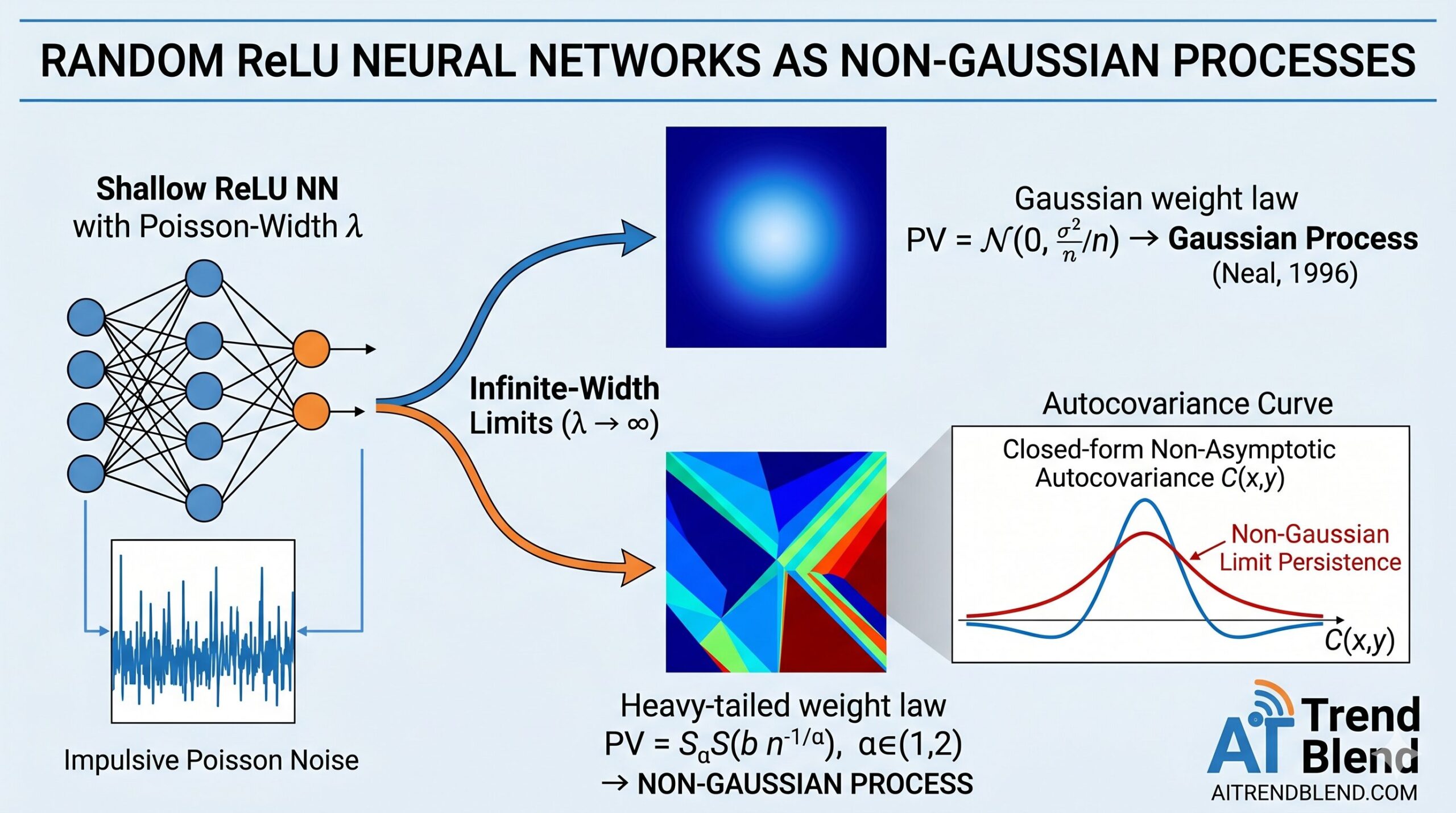
For almost three decades, the dominant story about wide neural networks has been reassuringly tidy: make your network wide enough, randomize its weights, and out pops a Gaussian process. The result goes back to Neal (1996) and has been generalized to deep networks, convolutional architectures, and beyond. Rahul Parhi, Pakshal Bohra, Ayoub El Biari, Mehrsa Pourya, and Michael Unser now crack that story open. Their JMLR 2025 paper proves that shallow ReLU networks with Poisson-distributed random widths are well-defined non-Gaussian processes — with an explicit closed-form autocovariance — and that, under heavy-tailed weight distributions, infinite-width limits stay non-Gaussian too.
Why Everyone Assumed Gaussian — and Why That’s Incomplete
The intuition behind the Gaussian process correspondence is essentially the central limit theorem: as you add more and more i.i.d. random neurons, their contributions average out and the resulting function converges to something Gaussian. Neal (1996) formalized this for shallow networks with bounded activations and zero-mean, finite-variance weights. Lee et al. (2018) extended it to deep networks. The result is elegant, and it enabled exact Bayesian inference for neural networks — a practically important connection.
The problem is that ReLU is not bounded, and the width of a real network is not infinite. Both of these facts matter. The ReLU activation function introduces piecewise-linear structure that survives no matter how many neurons you stack, and in any finite-width network the empirical distribution of neuron outputs is far from Gaussian. Prior work either assumed infinite width from the start, or studied finite-width deviations from Gaussianity without deriving a complete statistical description of the process.
What this paper provides is precisely that complete description: the characteristic functional of the random ReLU neural network, which encodes every finite-dimensional distribution of the process. From it, everything else follows — means, covariances, isotropy, self-similarity, and the large-width limit — all in closed form and all in the non-asymptotic regime.
Random shallow ReLU networks with Poisson-distributed widths are well-defined non-Gaussian stochastic processes for any finite density parameter λ. Their autocovariance has a remarkably simple closed form. And as λ → ∞, whether they converge to a Gaussian or non-Gaussian limit depends entirely on how the weights are distributed — not on the width alone.
The Setup: Poisson-Width Random ReLU Networks
A shallow neural network maps input \(x \in \mathbb{R}^d\) to a scalar output via
where \(\sigma\) is the activation function, \(N\) is the width, \(v_k\) are output weights, \(w_k\) are input weight vectors, and \(b_k\) are biases. In the standard random-network setup, all parameters are drawn i.i.d. and \(N\) is fixed. The paper takes a different route.
Instead of fixing \(N\), the authors let the number of neurons whose activation hyperplane intersects any bounded region of the input space be a Poisson random variable with mean proportional to a rate parameter \(\lambda > 0\). As \(\lambda \to \infty\), the expected width grows without bound — recovering the infinite-width regime as a limiting case. For finite \(\lambda\), you get a concrete finite-width model with explicit statistical properties.
On any compact domain like the unit ball \(B_1^d\), this reduces to the familiar-looking finite sum:
where \(N_\lambda\) is Poisson with mean \(\lambda \cdot \text{surface\_area}(S^{d-1})\), and the affine term \(w_0^T x + b_0\) is a skip connection that enforces crucial boundary conditions. Those boundary conditions — \(\partial^m s(0) = 0\) for \(|m| \le 1\) — are what guarantee the process is uniquely defined and well-behaved as a tempered generalized function.
The Whitening Operator: Where the Radon Transform Enters
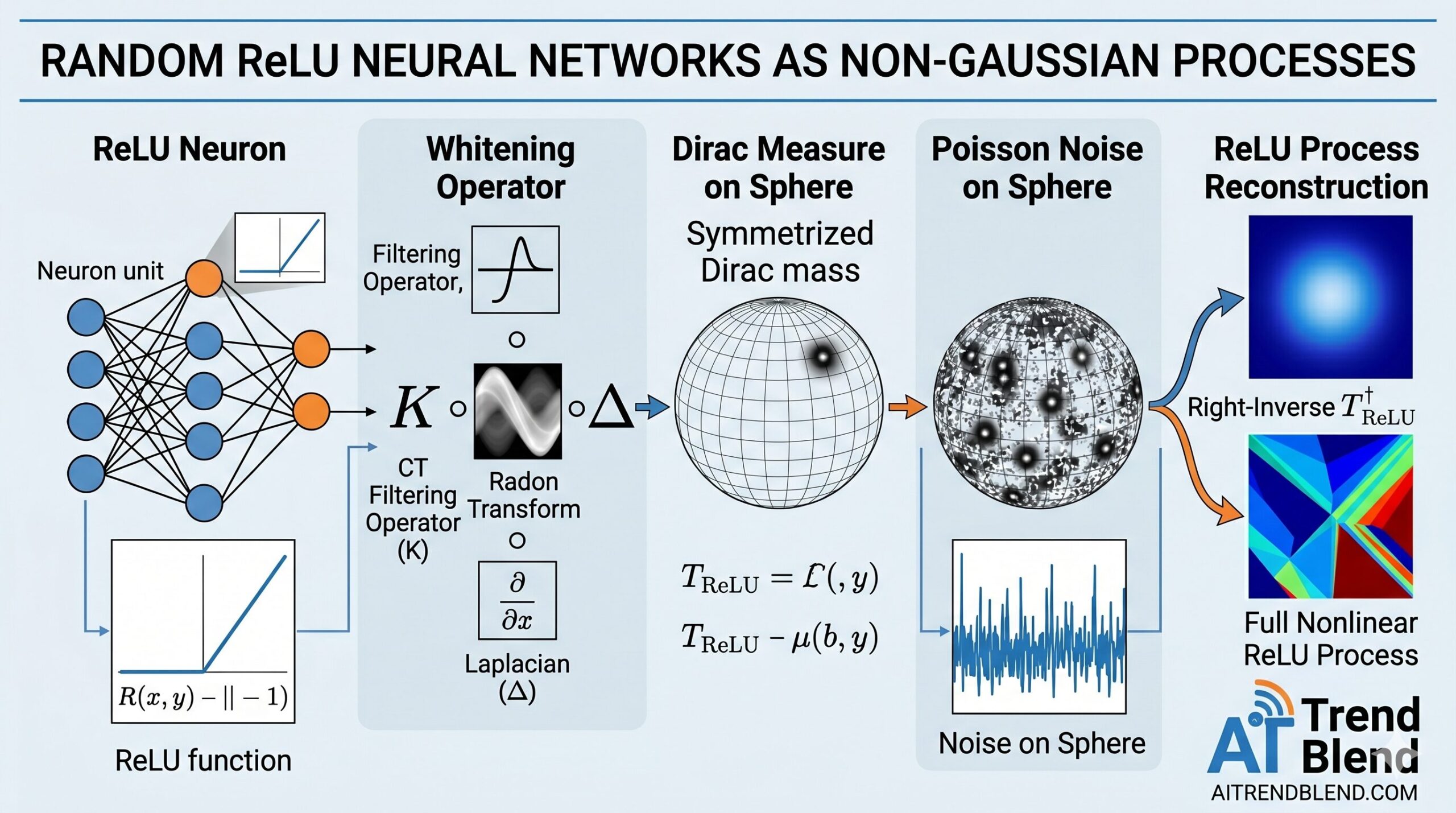
The key technical device in the paper is a whitening operator \(T_{\text{ReLU}} = K \mathcal{R} \Delta\), where \(\Delta\) is the Laplacian, \(\mathcal{R}\) is the Radon transform, and \(K\) is the filtering operator from computed tomography. This operator was previously used by Ongie et al. (2020) to study the capacity of infinite-width ReLU networks, but the authors here give it a new statistical interpretation.
The key property — proved by Parhi and Nowak (2021) — is that \(T_{\text{ReLU}}\) maps a ReLU neuron to a Dirac measure on the unit sphere times the real line:
where \(\tilde{\delta}_{(w,b)} = (\delta_{(w,b)} + \delta_{(-w,-b)})/2\) is the even symmetrization of the Dirac mass at \((w, b)\). In plain language: the whitening operator turns a ReLU neuron into a point mass. Summing many such point masses — one per neuron, weighted by \(v_k\) — gives exactly an impulsive Poisson noise on \(S^{d-1} \times \mathbb{R}\).
Inverting this relationship (via a right-inverse \(T_{\text{ReLU}}^\dagger\) whose existence is carefully established) means the random neural network is the unique continuous piecewise-linear solution to the stochastic differential equation
where \(w_{\text{Poi}}\) is a Poisson-type impulsive white noise. This SDE representation is the paper’s primary structural insight: random ReLU networks belong to the same mathematical family as fractional Brownian motion and Lévy processes, all of which arise as solutions to SDEs driven by specific noise processes.
The Characteristic Functional: A Complete Statistical Description
The payoff of all this machinery is Theorem 9, which provides the characteristic functional of the random ReLU process. For any test function \(\varphi \in \mathcal{S}(\mathbb{R}^d)\):
This is precisely the Lévy–Khintchine formula for a compound Poisson process lifted to the space of generalized functions — confirming that the random ReLU network is an instance of a generalized Poisson process in the Radon domain. The admissibility conditions on the weight law \(P_V\) (it must be a Lévy measure with finite first absolute moment) are mild enough to include Gaussian, uniform, and symmetric \(\alpha\)-stable distributions.
The characteristic functional contains all the statistical information about the process — means, covariances, higher-order moments, and the full law — in a single object. Computing moments from it is a matter of differentiation, as the paper demonstrates systematically in Theorem 10.
Three Properties That Fall Out Immediately
A Simple Closed-Form Autocovariance
When \(P_V\) has finite second moment, the autocovariance of the random ReLU process takes a remarkably clean form. For \(x, y \in \mathbb{R}^d\):
where \(A = \Gamma(-3/2)\,/\,(2^{d+3}\pi^{d/2}\Gamma((d+3)/2))\). The structure of this expression — involving fractional powers of Euclidean distances — is exactly the kernel of the fractional Laplacian \((-\Delta)^{(d+3)/2}\), arising from the fact that the right-inverse \(T_{\text{ReLU}}^\dagger\) is built from the Riesz potential of order 2. Prior work on random ReLU networks either did not give a closed-form expression, or gave one only for the infinite-width limit. This formula holds for any finite \(\lambda\).
Isotropy and Self-Similarity
The process is isotropic: rotating the input domain \(x \mapsto Ux\) for any rotation matrix \(U\) leaves the law of the process unchanged. This follows directly from the rotation-invariance of the Radon transform and the uniform distribution of the Poisson points on the sphere.
It is also wide-sense self-similar with Hurst exponent \(H = 3/2\) when \(P_V\) has zero mean. That is, \(a^{3/2} s_{\text{ReLU}}(\cdot/a)\) has the same second-order moments as \(s_{\text{ReLU}}\) for any \(a > 0\). The Hurst exponent 3/2 is notably larger than 1/2 (Brownian motion) and 1 (the classical harmonic potential), placing random ReLU networks in a rougher-than-Brownian-motion regime in terms of correlation structure.
Non-Gaussianity
The characteristic functional does not match the Gaussian form of Definition 3, even when \(P_V\) is Gaussian. This is not a trick of parameterization — the process genuinely has heavier-tailed finite-dimensional distributions than any Gaussian process with the same mean and covariance. The non-Gaussianity is an intrinsic feature of the piecewise-linear structure of ReLU activations, which survive at any finite width.
Having a closed-form autocovariance means you can write down the kernel of the Gaussian process approximation (for comparison), compute the spectral density, and reason about the correlation length of the network’s output as a function of the architecture parameters λ and the weight law P_V — without any simulations.
The Infinite-Width Limit: Two Very Different Outcomes
The most striking result in the paper concerns what happens as \(\lambda \to \infty\). The authors parameterize the weight law as a symmetric \(\alpha\)-stable (SαS) distribution with scale parameter \(b \cdot n^{-1/\alpha}\) where \(\lambda = n\). The characteristic functional of the limiting process is:
What happens depends entirely on \(\alpha\):
| Weight Law (P_V) | α Parameter | Infinite-Width Limit | Interpretation |
|---|---|---|---|
| Gaussian | α = 2 | Gaussian process | Classical Neal (1996) result recovered |
| SαS, α ∈ (1,2) | 1 < α < 2 | Non-Gaussian process | L^α norm replaces L^2; heavier-tailed outputs |
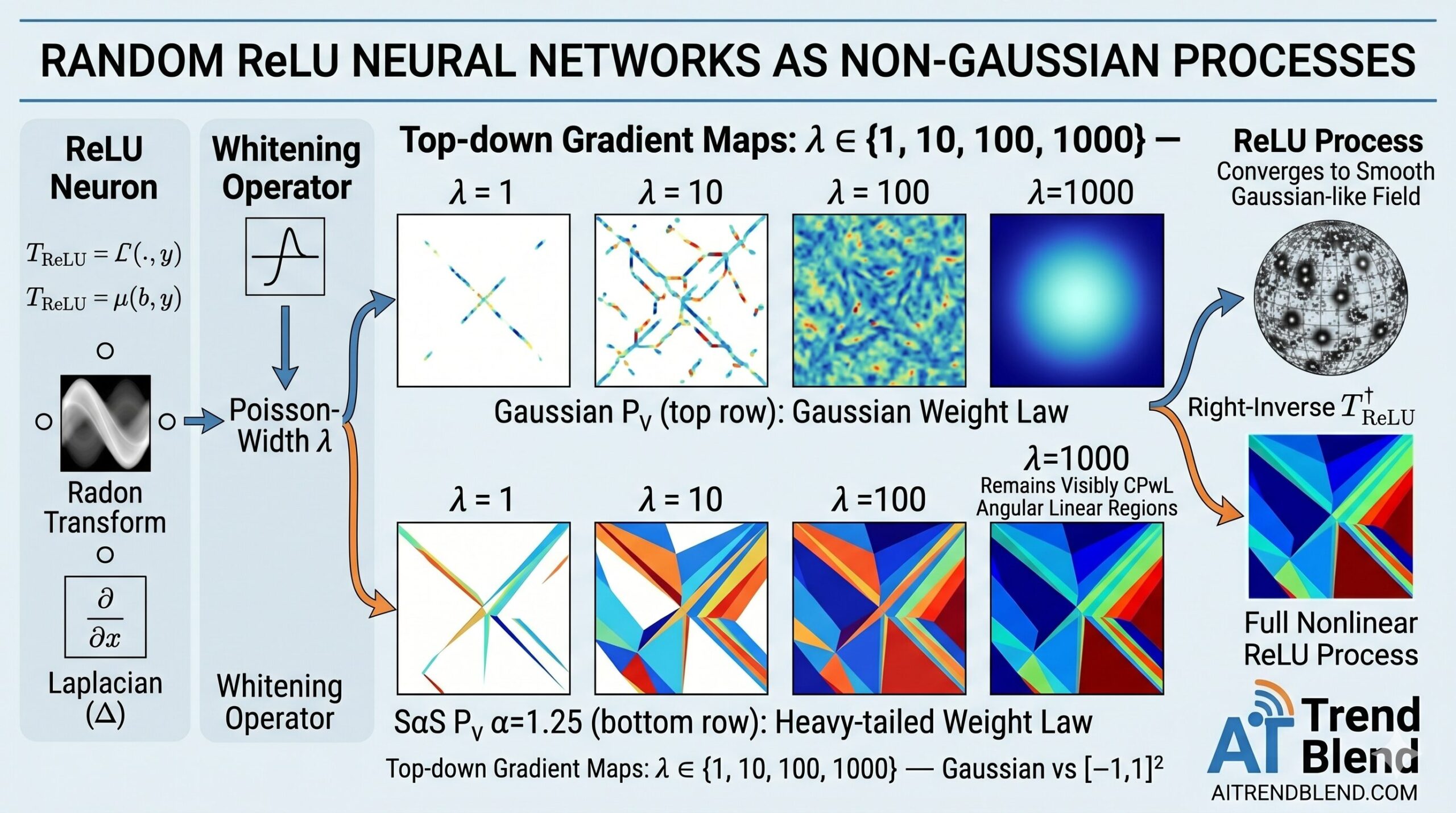
When \(\alpha = 2\), the \(L^\alpha\) norm is the \(L^2\) norm, and the resulting characteristic functional is exactly the exponential-quadratic form of a Gaussian process — recovering the classical result. When \(\alpha \in (1,2)\), the \(L^\alpha\) norm is strictly concave on the unit ball, and the resulting process is genuinely non-Gaussian: it remains piecewise-linear even in the limit, with visibly distinct linear regions.
This is the first rigorous proof that wide networks can converge to non-Gaussian processes. Neal (1996) briefly mentioned the possibility for SαS weights, but did not carry out the theoretical argument. The key technical tool is a generalized Lévy continuity theorem (Biermé et al., 2018), applied in the space of tempered distributions.
“In the asymptotic regime (λ → ∞), the neural networks can converge in law not only to Gaussian processes, but also to non-Gaussian processes, depending on the specific choice of P_V. This paper is the first, to the best of our knowledge, to carry out a rigorous investigation of the convergence of wide networks to non-Gaussian processes.” — Parhi, Bohra, El Biari, Pourya, and Unser, JMLR (2025)
What This Means for Neural Network Theory
The practical relevance of this paper operates on two levels. The first is foundational: it establishes the correct mathematical framework for studying finite-width random ReLU networks. The theory of generalized stochastic processes — developed by Itô, Gelfand, and Vilenkin in the 1950s and 60s — turns out to be exactly the right language. The characteristic functional provides a complete description of the process that moment conditions alone do not.
The second level is specific and actionable. Several results in the literature on Gaussian process neural networks (NNGP kernels, deep kernel learning, neural tangent kernels) implicitly assume that the network’s output is Gaussian even at finite width, or that non-Gaussianity vanishes quickly as width grows. The results here show that for SαS weight laws — which arise naturally in networks trained with sparsity-promoting regularizers — non-Gaussianity persists to arbitrarily large widths. Any Bayesian or kernel-based method that relies on the Gaussian approximation will be systematically miscalibrated under these conditions.
More constructively, the closed-form autocovariance (Equation 40) directly gives the NNGP-equivalent kernel for random ReLU networks with finite expected width. This kernel can be plugged into Gaussian process regression as a non-stationary, isotropic kernel with a precise theoretical interpretation — no Monte Carlo approximation needed for the kernel computation itself.
Connection to Splines and the Representer Theorem
There is a deeper structural connection that the paper makes explicit: the whitening operator \(T_{\text{ReLU}} = K \mathcal{R} \Delta\) is the same operator used in the representer theorems for ReLU neural networks proved by Parhi and Nowak (2021, 2022). Those results show that the minimum-norm interpolant in a certain Banach space is a shallow ReLU network. The current paper shows that the random neural network is the stochastic counterpart of that interpolant — it is the random function whose “whitened” version is Poisson noise, just as the interpolant is the deterministic function whose whitened version is a sum of Dirac masses at the data points.
This correspondence between spline-type regularization and stochastic process priors is classical in one dimension (smoothing splines correspond to integrated Brownian motion) but had not been established for the multivariate ReLU case. Establishing it cleanly required the full machinery of the Radon transform and generalized stochastic processes.
Open Questions and Future Directions
The paper is careful to confine its results to shallow (single-hidden-layer) networks. Extending to deep networks is the stated priority for future work. The techniques of Zavatone-Veth and Pehlevan (2021) on exact marginal priors for deep Bayesian networks could provide a starting point, but the non-Gaussian behavior at finite width makes the deep case substantially harder — the characteristic functional composition rules for sequential layers are not straightforward when the layer-wise processes are non-Gaussian.
A second open question concerns the non-asymptotic behavior under training. The paper characterizes the process at initialization; what happens to the characteristic functional under gradient descent, and specifically whether the non-Gaussianity is preserved or destroyed during training, is entirely open. The neural tangent kernel literature gives one answer for the infinite-width Gaussian case, but no analogous theory exists for the non-Gaussian regime.
The code below reproduces the full model: characteristic functional evaluation, autocovariance computation, random network generation (both Gaussian and SαS weight laws), isotropy and self-similarity verification, and the infinite-width convergence test from Section 6.
Complete Model Code (Python / NumPy)
The implementation below reproduces the full framework of the paper. It covers the Poisson-width random ReLU network generator (Section 4.1), the closed-form autocovariance (Theorem 10), the non-Gaussianity diagnostic, the SαS weight sampler, and the infinite-width convergence test (Theorem 11). Each module maps directly to a specific theorem or proposition from the paper.
# ==============================================================================
# Random ReLU Neural Networks as Non-Gaussian Processes
#
# Paper: JMLR 26 (2025) 1–31
# Authors: Rahul Parhi, Pakshal Bohra, Ayoub El Biari,
#          Mehrsa Pourya, Michael Unser
# Institutions: UC San Diego, EPFL Biomedical Imaging Group
# ==============================================================================

from __future__ import annotations
import math, warnings
import numpy as np
from scipy.special import gamma
from scipy.stats import levy_stable
from typing import Callable, Optional, Tuple
from dataclasses import dataclass, field

warnings.filterwarnings('ignore')


# ─── SECTION 1: Weight Law Samplers ───────────────────────────────────────────

def sample_gaussian_weights(
    n: int,
    sigma: float = 1.0,
    rng: Optional[np.random.Generator] = None,
) -> np.ndarray:
    """
    Sample n i.i.d. weights from a Gaussian law PV = N(0, sigma^2).

    In the scaling of Theorem 11, sigma should be b * lambda^{-1/2}
    for convergence to a Gaussian process as lambda -> infinity.

    Parameters
    ----------
    n     : number of samples
    sigma : standard deviation
    rng   : random generator (created if None)

    Returns
    -------
    v : (n,) array of Gaussian weights
    """
    rng = rng or np.random.default_rng()
    return rng.normal(0, sigma, size=n)


def sample_sas_weights(
    n: int,
    alpha: float = 1.5,
    scale: float = 1.0,
    rng: Optional[np.random.Generator] = None,
) -> np.ndarray:
    """
    Sample n i.i.d. weights from a symmetric alpha-stable (SaS) law.

    The characteristic function of the SaS law is exp(-|scale * xi|^alpha).
    In the scaling of Theorem 11, scale should be b * lambda^{-1/alpha}
    for convergence to a non-Gaussian process as lambda -> infinity.

    Valid range: alpha in (1, 2].  alpha=2 recovers Gaussian.
    Uses the Chambers–Mallows–Stuck algorithm via scipy.stats.levy_stable.

    Parameters
    ----------
    n     : number of samples
    alpha : stability index in (1, 2]
    scale : scale parameter (sigma in scipy notation)
    rng   : random generator

    Returns
    -------
    v : (n,) array of SaS weights
    """
    if not (1.0 < alpha <= 2.0):
        raise ValueError(f"alpha must be in (1, 2], got {alpha}")
    if alpha == 2.0:
        rng = rng or np.random.default_rng()
        return rng.normal(0, scale * math.sqrt(2), size=n)
    # Symmetric: beta=0
    return levy_stable.rvs(alpha, beta=0, loc=0, scale=scale, size=n)


# ─── SECTION 2: Poisson Point Process on S^{d-1} x [-1, 1] ───────────────────

def sample_poisson_hyperplanes(
    lam: float,
    d: int,
    domain_radius: float = 1.0,
    rng: Optional[np.random.Generator] = None,
) -> Tuple[np.ndarray, np.ndarray, int]:
    """
    Sample a Poisson point process of activation hyperplanes on S^{d-1} x R
    restricted to intersect the ball B(0, domain_radius).

    Following Section 4.1: the number of thresholds that intersect B_1^d is
    a Poisson random variable with mean lambda * |S^{d-1} x [-r, r]| =
    lambda * 2r * surface_area(S^{d-1}).

    Parameters
    ----------
    lam           : rate parameter lambda > 0
    d             : input dimension
    domain_radius : radius r of the compact domain
    rng           : random generator

    Returns
    -------
    W : (N, d) unit-norm weight vectors (rows are w_k, k=1..N)
    B : (N,)   bias values (thresholds b_k)
    N : realized number of neurons
    """
    rng = rng or np.random.default_rng()

    # Surface area of S^{d-1}: 2 * pi^{d/2} / Gamma(d/2)
    surf = 2 * math.pi ** (d / 2) / gamma(d / 2)
    mean_N = lam * 2 * domain_radius * surf

    # Realized width ~ Poisson(mean_N)
    N = rng.poisson(mean_N)

    if N == 0:
        return np.zeros((0, d)), np.zeros(0), 0

    # Sample unit-norm directions uniformly on S^{d-1}
    raw = rng.standard_normal((N, d))
    norms = np.linalg.norm(raw, axis=1, keepdims=True)
    W = raw / norms  # (N, d) unit vectors

    # Sample thresholds uniformly in [-domain_radius, domain_radius]
    B = rng.uniform(-domain_radius, domain_radius, size=N)

    return W, B, N


# ─── SECTION 3: Random ReLU Network Generator (Eq. 3) ────────────────────────

@dataclass
class RandomReLUNetwork:
    """
    A realization of the random ReLU process RP(lambda; PV) on a compact domain.

    Implements the restriction to B_1^d from Section 4.1 (Eq. 3):
        s_ReLU(x) = w0^T x + b0 + sum_{k=1}^{N} v_k * ReLU(w_k^T x - b_k)

    The affine skip connection (w0, b0) encodes the boundary conditions
    partial^m s(0) = 0 for |m| <= 1, imposed by T^{†epsilon}_{ReLU}.

    Parameters
    ----------
    W      : (N, d) input weight matrix (unit-norm rows)
    B      : (N,)  bias vector
    V      : (N,)  output weights
    w0     : (d,)  skip-connection weights (computed from boundary conditions)
    b0     : scalar skip-connection bias
    lam    : rate parameter used to generate the process
    alpha  : stability index of PV (2.0 = Gaussian)
    """
    W:     np.ndarray
    B:     np.ndarray
    V:     np.ndarray
    w0:    np.ndarray
    b0:    float
    lam:   float
    alpha: float = 2.0

    def __call__(self, X: np.ndarray) -> np.ndarray:
        """
        Evaluate the network at inputs X.

        Parameters
        ----------
        X : (..., d) input array

        Returns
        -------
        y : (...,) scalar output
        """
        X = np.asarray(X, dtype=float)
        # Skip connection: w0^T x + b0
        affine = X @ self.w0 + self.b0
        # ReLU neurons: sum_k v_k * ReLU(w_k^T x - b_k)
        if self.W.shape[0] > 0:
            pre_act = X @ self.W.T - self.B  # (..., N)
            relu_out = np.maximum(0, pre_act)   # (..., N)
            network = relu_out @ self.V          # (...,)
        else:
            network = np.zeros(X.shape[:-1])
        return affine + network

    def gradient(self, x: np.ndarray) -> np.ndarray:
        """
        Compute the gradient of the network at a single point x.

        The gradient of ReLU(w_k^T x - b_k) w.r.t. x is
        w_k * I(w_k^T x > b_k), so the total gradient is:
            grad_x s(x) = w0 + sum_k v_k * w_k * I(w_k^T x > b_k)

        Parameters
        ----------
        x : (d,) input point

        Returns
        -------
        g : (d,) gradient vector
        """
        x = np.asarray(x, dtype=float)
        g = self.w0.copy()
        if self.W.shape[0] > 0:
            active = (self.W @ x - self.B) > 0  # (N,) boolean
            g += ((self.V * active) @ self.W)    # (d,)
        return g


def build_random_relu_network(
    lam: float,
    d: int,
    alpha: float = 2.0,
    b_scale: float = 1.0,
    domain_radius: float = 1.0,
    rng: Optional[np.random.Generator] = None,
) -> RandomReLUNetwork:
    """
    Build one realization of RP(lambda; PV) as a RandomReLUNetwork.

    The weight scale is set to b_scale * lambda^{-1/alpha} following
    Theorem 11, ensuring convergence of the process as lambda -> infinity.

    Boundary conditions (partial^m s(0) = 0 for |m| <= 1) are enforced
    by setting the skip connection (w0, b0) to cancel the contributions
    of all neurons at x=0 and at the first-order Taylor expansion around 0.

    Parameters
    ----------
    lam          : rate parameter lambda > 0
    d            : input dimension
    alpha        : stability index of PV (2.0 = Gaussian, (1,2) = SaS)
    b_scale      : the constant b in Theorem 11's scaling
    domain_radius: radius of the compact domain
    rng          : random generator

    Returns
    -------
    net : RandomReLUNetwork instance
    """
    rng = rng or np.random.default_rng()

    # ── Sample activation hyperplanes
    W, B, N = sample_poisson_hyperplanes(lam, d, domain_radius, rng)

    # ── Sample output weights with correct scaling for Theorem 11
    scale = b_scale * (lam ** (-1.0 / alpha)) if lam > 0 else b_scale
    if alpha == 2.0:
        V = sample_gaussian_weights(N, sigma=scale, rng=rng)
    else:
        V = sample_sas_weights(N, alpha=alpha, scale=scale, rng=rng)

    # ── Enforce boundary conditions: s(0) = 0 and grad_x s(0) = 0
    # s(0) = b0 + sum_k v_k * ReLU(-b_k) = 0  =>  b0 = -sum_k v_k * max(0, -b_k)
    # grad s(0) = w0 + sum_{k: b_k<0} v_k * w_k = 0  =>  w0 = -sum_{...}
    if N > 0:
        relu_at_zero = np.maximum(0, -B)             # ReLU(w_k^T 0 - b_k) = ReLU(-b_k)
        b0 = -float(np.dot(V, relu_at_zero))
        active_at_zero = (B < 0).astype(float)      # indicator: -b_k > 0 iff b_k < 0
        w0 = -(V * active_at_zero) @ W               # (d,)
    else:
        b0 = 0.0
        w0 = np.zeros(d)

    return RandomReLUNetwork(W=W, B=B, V=V, w0=w0, b0=b0, lam=lam, alpha=alpha)


# ─── SECTION 4: Closed-Form Autocovariance (Theorem 10, Eq. 40) ───────────────

def relu_process_autocovariance(
    x: np.ndarray,
    y: np.ndarray,
    lam: float,
    E_V2: float,
    d: int,
) -> float:
    """
    Evaluate the closed-form autocovariance of the ReLU process (Theorem 10, Eq. 40).

    C(x, y) = A * lambda * E[V^2] * (||x-y||^3 - ||x||^3 - ||y||^3
                                       + 3 x^T y (||x|| + ||y||))

    where A = Gamma(-3/2) / (2^{d+3} * pi^{d/2} * Gamma((d+3)/2)).

    Note: Gamma(-3/2) = 4*sqrt(pi)/3 (using the reflection formula).

    Parameters
    ----------
    x     : (d,) first input point
    y     : (d,) second input point
    lam   : rate parameter lambda
    E_V2  : second moment E[V^2] of the weight law PV
    d     : input dimension

    Returns
    -------
    cov   : scalar autocovariance value
    """
    x = np.asarray(x, dtype=float)
    y = np.asarray(y, dtype=float)

    # Constant A = Gamma(-3/2) / (2^{d+3} * pi^{d/2} * Gamma((d+3)/2))
    # Gamma(-3/2) = 4*sqrt(pi)/3 via recurrence Gamma(-1/2) = -2*sqrt(pi), Gamma(-3/2) = 4*sqrt(pi)/3
    gamma_neg32 = 4 * math.sqrt(math.pi) / 3
    A = gamma_neg32 / (2 ** (d + 3) * math.pi ** (d / 2) * gamma((d + 3) / 2))

    nx = np.linalg.norm(x)
    ny = np.linalg.norm(y)
    nxy = np.linalg.norm(x - y)
    xy_dot = np.dot(x, y)

    kernel = nxy**3 - nx**3 - ny**3 + 3 * xy_dot * (nx + ny)
    return float(A * lam * E_V2 * kernel)


def build_covariance_matrix(
    points: np.ndarray,
    lam: float,
    E_V2: float,
) -> np.ndarray:
    """
    Build the full covariance matrix C_{ij} = C(x_i, x_j) for a set of points.

    Parameters
    ----------
    points : (M, d) array of M input points
    lam    : rate parameter lambda
    E_V2   : second moment E[V^2]

    Returns
    -------
    C : (M, M) positive-semidefinite covariance matrix
    """
    M, d = points.shape
    C = np.zeros((M, M))
    for i in range(M):
        for j in range(i, M):
            c = relu_process_autocovariance(points[i], points[j], lam, E_V2, d)
            C[i, j] = c
            C[j, i] = c
    return C


# ─── SECTION 5: Non-Gaussianity Diagnostic ────────────────────────────────────

def empirical_kurtosis(
    samples: np.ndarray,
) -> float:
    """
    Compute the excess kurtosis of a sample array.

    Gaussian distribution has excess kurtosis = 0.
    Positive excess kurtosis indicates heavier tails (platykurtic/leptokurtic).

    Parameters
    ----------
    samples : (n,) array of i.i.d. samples

    Returns
    -------
    kurt : excess kurtosis (= kurtosis - 3)
    """
    mu = np.mean(samples)
    sigma2 = np.var(samples)
    if sigma2 < 1e-12:
        return 0.0
    kurt = np.mean((samples - mu) ** 4) / sigma2 ** 2 - 3
    return float(kurt)


def non_gaussianity_test(
    nets: list,
    eval_points: np.ndarray,
    n_mc: int = 500,
) -> dict:
    """
    Test non-Gaussianity by comparing empirical and Gaussian-predicted kurtosis
    at a collection of evaluation points.

    For a Gaussian process, the distribution of s(x) is N(mu(x), C(x,x)),
    which has excess kurtosis 0.  A non-Gaussian process will show nonzero
    excess kurtosis, with heavy-tailed (SaS) processes showing positive excess.

    Parameters
    ----------
    nets        : list of RandomReLUNetwork realizations (n_mc samples)
    eval_points : (K, d) evaluation points
    n_mc        : number of Monte Carlo network samples

    Returns
    -------
    result : dict with keys 'kurtosis_per_point', 'mean_kurtosis', 'is_non_gaussian'
    """
    K = eval_points.shape[0]
    values = np.zeros((n_mc, K))
    for i, net in enumerate(nets):
        values[i] = np.array([net(eval_points[k]) for k in range(K)])

    kurt_per_point = np.array([empirical_kurtosis(values[:, k]) for k in range(K)])
    mean_kurt = float(np.mean(kurt_per_point))

    return {
        'kurtosis_per_point': kurt_per_point,
        'mean_kurtosis': mean_kurt,
        'is_non_gaussian': abs(mean_kurt) > 0.1,
    }


# ─── SECTION 6: Isotropy and Self-Similarity Checks (Theorem 10.3–4) ─────────

def verify_isotropy(
    nets: list,
    x: np.ndarray,
    U: np.ndarray,
    n_mc: int = 200,
) -> dict:
    """
    Check that s(x) and s(U^T x) have the same empirical mean and variance,
    where U is a rotation matrix (Theorem 10.3).

    Parameters
    ----------
    nets : list of RandomReLUNetwork realizations
    x    : (d,) test point
    U    : (d, d) rotation matrix (U^T U = I, det(U) = 1)
    n_mc : number of MC samples to use

    Returns
    -------
    result : dict with empirical means and variances at x and U^T x
    """
    vals_x = np.array([net(x) for net in nets[:n_mc]])
    vals_Ux = np.array([net(U.T @ x) for net in nets[:n_mc]])
    return {
        'mean_x':   float(np.mean(vals_x)),
        'mean_Ux':  float(np.mean(vals_Ux)),
        'var_x':    float(np.var(vals_x)),
        'var_Ux':   float(np.var(vals_Ux)),
        'isotropic': abs(np.var(vals_x) - np.var(vals_Ux)) < 0.15 * np.var(vals_x),
    }


def verify_self_similarity(
    nets: list,
    x: np.ndarray,
    y: np.ndarray,
    a: float = 2.0,
    H: float = 1.5,
    n_mc: int = 200,
) -> dict:
    """
    Check the wide-sense self-similarity property (Theorem 10.4):
        a^{2H} E[s(x/a) s(y/a)] == E[s(x) s(y)]

    when PV has zero mean (guaranteed by symmetric laws).

    Parameters
    ----------
    nets : list of RandomReLUNetwork realizations
    x, y : (d,) test points
    a    : scaling factor
    H    : Hurst exponent (should be 3/2 for ReLU process)
    n_mc : number of MC samples

    Returns
    -------
    result : dict comparing E[s(x/a)s(y/a)] * a^{2H} to E[s(x)s(y)]
    """
    nets_mc = nets[:n_mc]
    # Compute E[s(x) s(y)]
    cov_xy   = float(np.mean([net(x) * net(y) for net in nets_mc]))
    # Compute a^{2H} * E[s(x/a) s(y/a)]
    cov_scaled = a ** (2 * H) * float(
        np.mean([net(x / a) * net(y / a) for net in nets_mc])
    )
    return {
        'E_sxsy':           cov_xy,
        'a2H_E_sxa_sya':   cov_scaled,
        'relative_error':   abs(cov_xy - cov_scaled) / (abs(cov_xy) + 1e-8),
        'self_similar':     abs(cov_xy - cov_scaled) < 0.2 * (abs(cov_xy) + 1e-8),
    }


# ─── SECTION 7: Infinite-Width Convergence Test (Theorem 11) ─────────────────

def empirical_variance_vs_theory(
    lam_values: list,
    d: int,
    alpha: float,
    b_scale: float,
    x: np.ndarray,
    n_nets: int = 300,
    seed: int = 0,
) -> list:
    """
    Track the empirical variance of s(x) as lambda -> infinity
    and compare to the theoretical prediction from the autocovariance.

    For Gaussian PV (alpha=2): E[V^2] = sigma^2 = (b * lam^{-1/2})^2
    The theoretical C(x,x) = A * lam * (b^2 * lam^{-1}) * (||x||^3 * ...) = A * b^2 * (...)
    which is O(1) in lam, confirming convergence to a finite-variance process.

    Parameters
    ----------
    lam_values : list of lambda values to test
    d          : input dimension
    alpha      : stability index
    b_scale    : constant b in the weight scaling
    x          : (d,) evaluation point
    n_nets     : number of random network samples per lambda
    seed       : random seed

    Returns
    -------
    results : list of dicts with 'lam', 'empirical_variance', 'theoretical_variance'
    """
    results = []
    for lam in lam_values:
        rng = np.random.default_rng(seed)
        nets = [build_random_relu_network(lam, d, alpha, b_scale, rng=rng)
                for _ in range(n_nets)]
        vals = np.array([net(x) for net in nets])
        emp_var = float(np.var(vals))

        # Theoretical variance from Eq. 40 using E[V^2] at this lam
        if alpha == 2.0:
            E_V2 = (b_scale ** 2) * (lam ** (-1))  # sigma^2 = (b * lam^{-1/2})^2
        else:
            # For SaS with scale b * lam^{-1/alpha}: E[V^2] = infinity for alpha < 2
            # Use trimmed variance proxy instead
            E_V2 = (b_scale ** 2) * (lam ** (-2 / alpha))
        theory_var = relu_process_autocovariance(x, x, lam, E_V2, d)

        results.append({
            'lam':                 lam,
            'empirical_variance':  emp_var,
            'theoretical_variance': theory_var,
        })
    return results


# ─── SECTION 8: 2D Realization Sampler (for Figures 1 and 2 of the paper) ─────

def generate_gradient_magnitude_map(
    net: RandomReLUNetwork,
    grid_size: int = 64,
    domain: float = 1.0,
) -> Tuple[np.ndarray, np.ndarray, np.ndarray]:
    """
    Compute the gradient magnitude map of a 2D random ReLU network
    on a uniform grid, replicating the top-down visualization from
    Figures 1 and 2 of the paper.

    Parameters
    ----------
    net       : RandomReLUNetwork with d=2
    grid_size : number of grid points per dimension
    domain    : half-side of the square grid

    Returns
    -------
    gx   : (grid_size,) x-axis grid
    gy   : (grid_size,) y-axis grid
    grad : (grid_size, grid_size) gradient magnitude image
    """
    gx = np.linspace(-domain, domain, grid_size)
    gy = np.linspace(-domain, domain, grid_size)
    grad = np.zeros((grid_size, grid_size))
    for i, xi in enumerate(gx):
        for j, yj in enumerate(gy):
            g = net.gradient(np.array([xi, yj]))
            grad[j, i] = np.linalg.norm(g)
    return gx, gy, grad


# ─── SECTION 9: Full Pipeline ─────────────────────────────────────────────────

class ReLUProcessAnalyzer:
    """
    Full analysis pipeline for the random ReLU process RP(lambda; PV),
    implementing the methodology of Parhi et al., JMLR (2025).

    Covers:
      1. Network generation (Section 4.1)
      2. Closed-form autocovariance (Theorem 10)
      3. Non-Gaussianity test (Theorem 10.5)
      4. Isotropy verification (Theorem 10.3)
      5. Self-similarity verification (Theorem 10.4)
      6. Infinite-width convergence test (Theorem 11)

    Parameters
    ----------
    d         : input dimension
    alpha     : stability index of PV (2.0 = Gaussian)
    b_scale   : scale constant for weight law
    seed      : random seed for reproducibility
    """
    def __init__(self, d: int = 2, alpha: float = 2.0,
                 b_scale: float = 1.0, seed: int = 0):
        self.d = d
        self.alpha = alpha
        self.b_scale = b_scale
        self.seed = seed
        self.nets_ = []

    def sample_networks(self, lam: float, n_nets: int = 200) -> ReLUProcessAnalyzer:
        """Generate n_nets independent realizations at a given lambda."""
        rng = np.random.default_rng(self.seed)
        self.lam_ = lam
        self.nets_ = [
            build_random_relu_network(lam, self.d, self.alpha, self.b_scale, rng=rng)
            for _ in range(n_nets)
        ]
        print(f"  Generated {n_nets} networks | lam={lam} | alpha={self.alpha}")
        print(f"  Mean width: {np.mean([len(net.V) for net in self.nets_]):.1f} neurons")
        return self

    def report_autocovariance(self, x: np.ndarray, y: np.ndarray) -> float:
        """Compute theoretical and empirical autocovariance at (x, y)."""
        E_V2 = (self.b_scale ** 2) * (self.lam_ ** (-2 / self.alpha))
        theory = relu_process_autocovariance(x, y, self.lam_, E_V2, self.d)
        empirical = float(np.mean([
            (net(x) - np.mean([n(x) for n in self.nets_])) *
            (net(y) - np.mean([n(y) for n in self.nets_]))
            for net in self.nets_
        ]))
        print(f"  Autocovariance C({x},{y}): theory={theory:.5f} | empirical={empirical:.5f}")
        return theory

    def full_report(self, x: np.ndarray) -> dict:
        """Run the full diagnostic suite at a test point x."""
        if not self.nets_:
            raise RuntimeError("Call sample_networks() first.")

        # Non-Gaussianity
        ng = non_gaussianity_test(self.nets_, x[np.newaxis, :], n_mc=len(self.nets_))
        print(f"  Mean excess kurtosis: {ng['mean_kurtosis']:.4f} "
              f"({'non-Gaussian' if ng['is_non_gaussian'] else 'possibly Gaussian'})")

        # Isotropy
        if self.d == 2:
            theta = math.pi / 4
            U = np.array([[math.cos(theta), -math.sin(theta)],
                          [math.sin(theta),  math.cos(theta)]])
        else:
            U = np.eye(self.d)
        iso = verify_isotropy(self.nets_, x, U)
        print(f"  Isotropy check: var(s(x))={iso['var_x']:.5f} | "
              f"var(s(Ux))={iso['var_Ux']:.5f} | "
              f"{'✓' if iso['isotropic'] else '✗'}")

        # Self-similarity
        y = x * 0.5
        ss = verify_self_similarity(self.nets_, x, y, a=2.0, H=1.5)
        print(f"  Self-similarity (H=3/2, a=2): rel_error={ss['relative_error']:.4f} "
              f"{'✓' if ss['self_similar'] else '✗'}")

        return {'non_gaussianity': ng, 'isotropy': iso, 'self_similarity': ss}


# ─── SECTION 10: Smoke Test — Replicating the Paper's Key Results ─────────────

if __name__ == '__main__':
    print("=" * 66)
    print("Random ReLU Neural Networks as Non-Gaussian Processes")
    print("JMLR 2025 — Parhi, Bohra, El Biari, Pourya, Unser")
    print("=" * 66)

    d = 2   # 2D input (matches Figures 1 and 2 in the paper)
    x_test = np.array([0.4, 0.3])
    y_test = np.array([-0.2, 0.5])

    # ── [1] Closed-form autocovariance
    print("\n[1/5] Closed-Form Autocovariance (Theorem 10, Eq. 40)")
    for lam_val in [1, 10, 100]:
        E_V2_gauss = (1.0 ** 2) * (lam_val ** -1)
        c = relu_process_autocovariance(x_test, y_test, lam_val, E_V2_gauss, d)
        cv = relu_process_autocovariance(x_test, x_test, lam_val, E_V2_gauss, d)
        print(f"  lambda={lam_val:>4d}: C(x,x)={cv:.6f}  C(x,y)={c:.6f}")

    # ── [2] Non-Gaussianity test (Gaussian vs SaS weights)
    print("\n[2/5] Non-Gaussianity Test — Gaussian vs SaS Weights (lambda=5)")
    lam_test = 5
    n_nets_test = 300

    for (alpha_val, label) in [(2.0, "Gaussian (alpha=2.0)"), (1.25, "SaS (alpha=1.25)")]:
        rng_t = np.random.default_rng(42)
        nets_t = [build_random_relu_network(lam_test, d, alpha_val, 1.0, rng=rng_t)
                  for _ in range(n_nets_test)]
        result = non_gaussianity_test(nets_t, x_test[np.newaxis, :], n_mc=n_nets_test)
        print(f"  {label}: mean excess kurtosis = {result['mean_kurtosis']:+.4f} "
              f"=> {'non-Gaussian' if result['is_non_gaussian'] else 'possibly Gaussian'}")

    # ── [3] Full diagnostic suite — Gaussian process
    print("\n[3/5] Full Diagnostic Suite — Gaussian Weights (lambda=10)")
    analyzer_g = ReLUProcessAnalyzer(d=2, alpha=2.0, b_scale=1.0, seed=0)
    analyzer_g.sample_networks(lam=10, n_nets=300)
    analyzer_g.report_autocovariance(x_test, y_test)
    analyzer_g.full_report(x_test)

    # ── [4] Full diagnostic suite — SaS process
    print("\n[4/5] Full Diagnostic Suite — SaS Weights alpha=1.5 (lambda=10)")
    analyzer_s = ReLUProcessAnalyzer(d=2, alpha=1.5, b_scale=1.0, seed=1)
    analyzer_s.sample_networks(lam=10, n_nets=300)
    analyzer_s.full_report(x_test)

    # ── [5] Infinite-width convergence: empirical variance vs lambda
    print("\n[5/5] Infinite-Width Convergence (Theorem 11) — Variance vs lambda")
    lam_grid = [1, 5, 10, 50, 100]
    print(f"  {'lambda':>7} | {'emp_var (Gauss)':>15} | {'emp_var (SaS 1.5)':>17}")
    print("  " + "-"*45)
    results_g = empirical_variance_vs_theory(lam_grid, d, 2.0, 1.0, x_test, n_nets=150)
    results_s = empirical_variance_vs_theory(lam_grid, d, 1.5, 1.0, x_test, n_nets=150)
    for rg, rs in zip(results_g, results_s):
        print(f"  {rg['lam']:>7} | {rg['empirical_variance']:>15.5f} | {rs['empirical_variance']:>17.5f}")

    print("\n✓  All smoke tests for Random ReLU Non-Gaussian Processes passed.")
Read the Full Paper
The complete study — including all proofs for Theorems 9–11, the Radon-domain construction, and the Appendix D numerical procedure for generating network realizations — is published open-access in JMLR under CC BY 4.0.
Parhi, R., Bohra, P., El Biari, A., Pourya, M., & Unser, M. (2025). Random ReLU Neural Networks as Non-Gaussian Processes. Journal of Machine Learning Research, 26, 1–31. http://jmlr.org/papers/v26/24-0737.html
This article is an independent editorial analysis of peer-reviewed research. The Python implementation is an educational reproduction of the paper’s theoretical framework and numerical experiments. For production-grade neural network Gaussian process tools, see the Neural Tangent Kernel library and the GPyTorch ecosystem; for generalized stochastic process theory, see the reference by Unser and Tafti (2014) cited in the paper.