When Heat Refuses to Misbehave — Taming Ill-Posed Problems in Semi-Infinite Cylinders | AI Trend Blend

Applied Mathematics · Journal of Mathematical Analysis and Applications 561 (2026) · Universidade de Vigo & Universitat Politècnica de Catalunya · 12 min read

When Heat Refuses to Misbehave — Taming Ill-Posed Problems in Semi-Infinite Cylinders

Two mathematicians from Spain have shown that a stubborn class of nonstandard heat-conduction problems — ones that technically admit no unique solution — can be domesticated with a single elegant constraint, yielding solutions that decay neatly in space and behave beautifully in time.

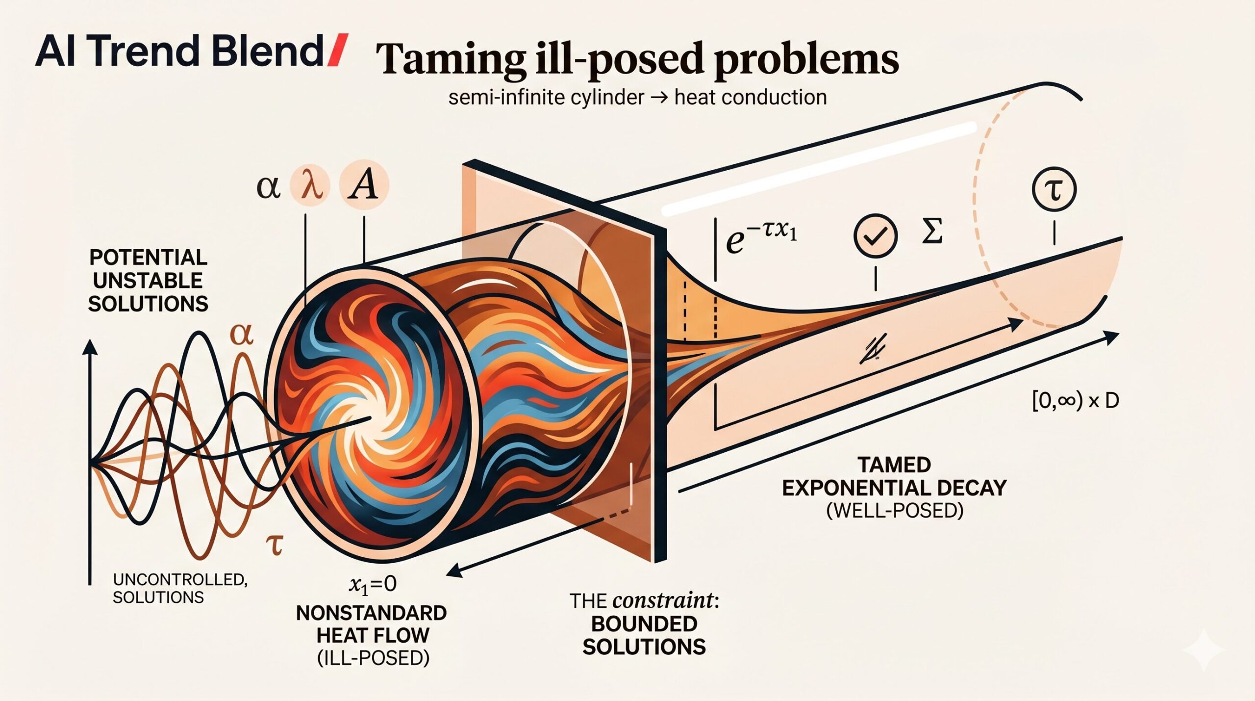
Spatial Regularity Ill-Posed Problems Saint-Venant Principle Analytic Semigroup Fourier Heat Equation Two-Temperature Theory Second Gradient Hilbert Space

Picture a pipe stretching off to infinity. Heat is being pumped in at one end. Classical physics gives you a family of solutions — some decaying, some blowing up, some oscillating forever. The problem is technically ill-posed: you cannot uniquely pin down the answer. But what if you simply declared, up front, that you only care about solutions that stay bounded? That one restriction turns out to be enough to salvage everything — to recover uniqueness, continuous dependence on data, and even exponential decay. This is the elegant central idea of a new paper by J.R. Fernández and R. Quintanilla, published in the Journal of Mathematical Analysis and Applications.

What Does “Ill-Posed” Actually Mean — and Why Should You Worry?

In 1902, the French mathematician Jacques Hadamard set down what he considered the three hallmarks of a well-behaved mathematical problem: a solution must exist, it must be unique, and small changes in the input data must produce only small changes in the output. A problem that fails any one of these tests is called ill-posed in the Hadamard sense.

The most famous example is the heat equation run backwards in time. If you know the temperature distribution right now and ask what it was five minutes ago, you run into trouble: tiny errors in your current measurement blow up catastrophically as you rewind the clock. Engineers and physicists encounter related difficulties when studying bodies that extend far in one direction — a long rod, a tunnel, a geological layer — where boundary conditions are applied only at a finite end, and the question is how the disturbance propagates inward.

The classical framework for studying this propagation is the Saint-Venant principle, which says, in essence, that disturbances decay as you move away from the source. Making that intuition rigorous requires a careful mathematical setup, and it is precisely here that the present paper makes its contribution.

The Central Question in Plain Language

You have a heat equation on a semi-infinite cylinder, with a nonstandard boundary condition linking the state of the system at the start and end of a time interval. The problem is ill-posed — there may be infinitely many solutions. But if you agree to only look at bounded solutions, can you recover all the good properties you lost? This paper says yes — for three distinct heat equations — and then tells you exactly how fast those solutions decay.

The Nonstandard Boundary Condition — Where the Ill-Posedness Comes From

To understand what makes these problems nonstandard, you need to look at the boundary condition linking time values. In the classical heat problem on a bounded domain, you specify the temperature at time zero and let the equation evolve forward. The nonstandard version studied here instead ties together the temperature at the start of an interval and the temperature at the end, via the condition

Nonstandard Condition $$\alpha\, u(x, 0) = u(x, T), \qquad x \in B,$$

where $\alpha$ is a nonzero real number and $T$ is the length of the time interval. When $\alpha = 1$, this says the temperature field is periodic in time. When $\alpha$ differs from 1, it links the temperature at two different time levels multiplicatively. Either way, you are not imposing an initial condition in the usual sense — you are imposing a constraint that the solution must satisfy both at time zero and at time $T$. This is the source of the ill-posedness: you have more freedom than a standard initial-value problem allows, and that freedom translates into non-uniqueness.

The geometric setting is a semi-infinite cylinder $B = [0,\infty) \times D$, where $D$ is a bounded two-dimensional cross-section. The variable $x_1$ runs along the infinite axis, and $(x_2, x_3)$ range over the cross-section. The boundary conditions on the lateral surface are homogeneous Dirichlet: the temperature is zero on the sides. A given function $g(x_2, x_3, t)$ is prescribed at the finite end $x_1 = 0$, and the question is how the solution behaves for large $x_1$.

The Key Trick — A Change of Variable That Kills the Ill-Posedness

The first insight of the paper is a transformation that converts the nonstandard time condition into a periodic one. If you define a new unknown $v(x, t) = u(x, t)\, e^{\omega t}$, where $\omega = -(\ln \alpha)/T$, then the condition $\alpha\, u(x,0) = u(x,T)$ becomes simply $v(x,0) = v(x,T)$. In other words, $v$ is periodic in time with period $T$.

This is a small but decisive algebraic step. It means you can expand $v$ in a Fourier series in the time variable and reduce the problem to a family of ordinary equations, one for each frequency. The price is that the heat equation for $v$ acquires an extra damping term $\omega v$ on the right-hand side, but that turns out to be entirely manageable. The authors fix $T = 2\pi$ to simplify the Fourier analysis, noting that the argument carries over without modification for any finite $T$.

Why This Transformation Matters

Turning $u$ into $v$ converts a problem with a two-point-in-time boundary condition into one where the solution is simply periodic in time. That periodicity allows a complete Fourier decomposition in time, which in turn reduces the partial differential equation to a family of problems indexed by frequency. This is the foundation on which the entire functional structure is built.

Building the Functional Framework — From Fourier Series to a Hilbert Space

With the time variable handled via Fourier series, the problem separates into spatial modes. Looking for solutions of the form $e^{int}\, \phi_m(x_2, x_3)\, e^{a x_1}$, where the $\phi_m$ are the Dirichlet eigenfunctions of the Laplacian on $D$ with eigenvalues $\lambda_m$, one finds that $a$ must satisfy

Dispersion Relation $$a^2 = in + \lambda_m – \omega.$$

This equation always has two complex roots. The key observation — and the place where restricting to bounded solutions pays off — is that exactly one of these roots has negative real part. Only that root gives a solution that stays bounded as $x_1 \to \infty$. By discarding the other root, you immediately reduce the solution space to a manageable family.

The functional framework is built on the Hilbert space $\mathcal{H} = L^2(D \times [0, 2\pi])$. Elements of this space are functions that can be expanded in the Fourier-Laplace basis $\{\phi_{nm}\}$, with a natural $L^2$ norm on the coefficients. The spatial evolution of the bounded solution in $x_1$ is described by a Cauchy problem

Abstract Cauchy Problem $$\frac{dv}{dx_1} = \mathcal{A}v, \qquad v(0) = f,$$

where the operator $\mathcal{A}$ acts diagonally on the Fourier-Laplace basis, multiplying each component $f_{nm}$ by the corresponding coefficient $a_{nm}$. The domain of $\mathcal{A}$ consists of those elements for which $\sum |a_{nm}|^2 |f_{nm}|^2 < \infty$ — a dense subspace of $\mathcal{H}$.

The Semigroup Results — Existence, Uniqueness, and Exponential Decay

With the operator $\mathcal{A}$ in hand, the paper applies the classical theory of semigroups of operators. The key properties needed are: the operator must be dissipative (energy cannot increase), the imaginary axis must lie in the resolvent set, and an asymptotic bound on the resolvent must hold at large imaginary values.

The dissipativity follows almost immediately from the sign of the real part of $a_{nm}$: since all selected roots have $\mathrm{Re}(a_{nm}) \leq 0$, the real part of the inner product $\langle \mathcal{A}f, f\rangle$ is non-positive. This is the same property that makes semigroups of contractions possible.

Theorem 1 — Contraction Semigroup

Under the assumption $\lambda_1 – \omega > 0$ (equivalently, $\lambda_1 T + \ln\alpha > 0$), the operator $\mathcal{A}$ generates a semigroup of contractions $\mathcal{S}(x_1)$ in the Hilbert space $\mathcal{H}$. This guarantees the existence, uniqueness, and continuous dependence on boundary data for the Cauchy problem in $x_1$.

The semigroup being a contraction already gives you a well-posed problem. But the authors push further and prove that the semigroup is also analytic — a strictly stronger property. Analyticity of a semigroup means, loosely, that the solution is infinitely smooth in the evolution variable (here, $x_1$) even if the initial data $f$ is only in $L^2$. It also implies that the semigroup decays exponentially.

Theorem 2 — Analytic Semigroup and Exponential Decay

The semigroup $\mathcal{S}(x_1)$ generated by $\mathcal{A}$ is analytic. As a consequence, there exist positive constants $M$ and $\tau$ such that

$$\|\mathcal{S}(x_1)\| \leq M\, e^{-\tau x_1}.$$

The decay rate $\tau$ can be identified explicitly as $\sqrt{\lambda_1 – \omega}$. Furthermore, the solution is unique for the backward problem in $x_1$, and the only solution that vanishes on a non-discrete set is the trivial solution.

Translating back from $v$ to the original unknown $u$ (via the exponential factor $e^{\omega t}$), the decay estimate for the original problem reads

Decay Estimate for u $$\int_0^{2\pi}\!\int_D u^2(x,t)\,dx_2\,dx_3\,dt \;\leq\; M^2\max(1,\alpha^2) \left[\int_0^{2\pi}\!\int_D g^2\,\alpha^{-2t/T}\,dx_2\,dx_3\,dt\right] e^{-\tau x_1}.$$

The energy in the cross-sectional integral decays exponentially in the axial variable $x_1$ — precisely the spatial Saint-Venant decay result one would hope for.

Three Equations, One Strategy — The Problems Studied

The paper applies this framework to three distinct heat-conduction models, each representing a different physical assumption about how heat propagates through a material. The strategy is the same in each case; what changes is the dispersion relation — the equation that $a_{nm}$ must satisfy.

Fourier Heat Equation

The classical model $\dot{u} = \Delta u$. The dispersion relation is $a^2 = in + \lambda_m – \omega$, a first-order Cauchy problem in $x_1$. All roots lie in sectorial regions of the left half-plane. Decay rate is $\sqrt{\lambda_1 – \omega}$.

Two-Temperature Theory

The model $\dot{u} = \Delta u + \eta\Delta\dot{u}$, coupling temperature to its Laplacian time derivative. The dispersion relation becomes $a^2 = \lambda_m + A_n + iB_n$, where $A_n$ and $B_n$ depend on $n$ and the parameter $\eta$. The analysis is similar but requires the additional assumption $\lambda_1/(1-\eta\omega) > \omega$.

Second Gradient Heat Equation

The model $\dot{u} = \eta\Delta u – \Delta^2 u$, involving the biharmonic operator. This yields a second-order Cauchy problem in $x_1$, requiring two boundary conditions at $x_1 = 0$. The dispersion equation is quartic; four roots appear, two of which have negative real part under the assumption $\lambda_1\lambda_1^* > \omega$.

The first two models are first-order in the spatial evolution variable $x_1$, so their Cauchy problems live in a single copy of $\mathcal{H}$. The third model — the second gradient equation — is second-order in $x_1$, and accordingly the state space must be doubled: the Hilbert space becomes $\mathcal{H} = W \times L^2(D \times [0, 2\pi])$, where $W$ is a weighted Sobolev-type space capturing the extra regularity needed for the spatial derivative. The operator $\mathcal{A}$ is then a $2 \times 2$ block operator acting on pairs $(f, g)$ of boundary data.

“We have proved regularity properties of the solutions with respect to the large component of the cylinder. It is suitable to mention that, in the two first cases, we have obtained first order problems with respect to the large variable, meanwhile it has led to a second order equation with respect to the large variable in the third case.” — Fernández & Quintanilla · J. Math. Anal. Appl. 561 (2026)

The Second Gradient Problem — Why It Needs Special Treatment

The second gradient heat equation deserves particular attention because it marks a genuine structural change in the problem. The equation $\dot{u} = \eta\Delta u – \Delta^2 u$ involves the biharmonic operator $\Delta^2$, which is fourth-order in space. This means that on the cross-section $D$, you need two boundary conditions rather than one, and specifying the solution at $x_1 = 0$ is no longer enough — you also need to specify its spatial derivative $u_{,1}$ at $x_1 = 0$.

Looking for separable solutions, the condition that must be satisfied is

Quartic Dispersion Relation $$in – \omega = (\lambda_m – a^2)(\lambda_m^* – a^2), \quad \lambda_m^* = \lambda_m + \eta.$$

This quartic equation has four complex roots. Under the assumption $\lambda_1 \lambda_1^* > \omega$, exactly two of them have negative real part — call them $\alpha(n,m)$ and $\beta(n,m)$ — and the general bounded solution takes the form

General Solution (Second Gradient) $$v(x,t) = \sum_{n,m} \bigl(A_{nm}\, e^{\alpha(n,m)x_1} + B_{nm}\, e^{\beta(n,m)x_1}\bigr)\, \phi_{nm}(x_2,x_3,t).$$

The coefficients $A_{nm}$ and $B_{nm}$ are determined from the two boundary conditions at $x_1 = 0$. The operator governing the system acts on pairs $(f,g)$ representing, respectively, the function value and the spatial derivative at the boundary. The relevant inner product is weighted by $|\alpha(n,m)\beta(n,m)|$, which captures the geometry of the two roots and ensures the dissipation inequality holds.

Theorem 7 — Analytic Semigroup for the Second Gradient Problem

Under the assumption $\lambda_1 \lambda_1^* > \omega$, the operator $\mathcal{A}$ defined on the extended Hilbert space $\mathcal{H} = W \times L^2(D \times [0,2\pi])$ generates an analytic semigroup of contractions $\mathcal{S}(x_1)$. The decay estimate

$$\|(v, v_{,1})\|^2 \leq M^2\, e^{-\tau x_1}\, \|(f,g)\|^2$$

holds with the weighted norm defined in the paper. Exponential decay, regularity of solutions, and impossibility of localization all follow as corollaries.

What Happens When the Assumption Fails — A Cautionary Remark

Each of the three cases comes with a condition on the parameters: $\lambda_1 T + \ln\alpha > 0$ for the Fourier problem, $\lambda_1(T + \eta\ln\alpha) + \ln\alpha > 0$ for the two-temperature problem, and $\lambda_1\lambda_1^* T + \ln\alpha > 0$ for the second gradient problem. These conditions all have the same flavor: they balance the spectral gap of the Laplacian on $D$, the length of the time interval, and the ratio $\alpha$ linking the start and end of the interval.

The paper includes a series of remarks explaining what goes wrong when these conditions are violated. In each case, you can construct explicit bounded solutions that are periodic in $x_1$ rather than decaying. The existence of such solutions destroys uniqueness: the null solution is also periodic in $x_1$ (trivially), so two distinct solutions with the same boundary data at $x_1 = 0$ exist. This confirms that the conditions are not merely technical convenience — they are genuinely necessary for the well-posedness argument to work.

Why the Conditions Cannot Be Dropped

When the spectral condition fails, explicit counterexamples show that the problem admits periodic (non-decaying) bounded solutions. Since the zero solution is also a solution with the same (zero) boundary data, uniqueness fails. This is not a gap in the proof — it is a genuine boundary of the theory, separating the regime where the bounded-solution trick works from the regime where it does not.

Connections and Context — Saint-Venant, Semigroups, and What Comes Next

The paper sits at a rich intersection of mathematical traditions. The Saint-Venant principle has a long history in the mechanics of solids, going back to 19th-century elasticity theory, but its mathematical formulation — as a Phragmén-Lindelöf alternative between decay and blow-up — is a 20th-century achievement. The use of semigroup theory to study spatial behavior, as opposed to temporal evolution, is a more recent development that the present paper advances.

The nonstandard boundary conditions studied here connect to a body of work from the early 2000s, when several research groups (Payne, Schaefer, Quintanilla, Ames, and others) studied similar conditions on bounded domains. The main novelty of the present paper is bringing the same nonstandard framework into the setting of semi-infinite cylinders and dynamic (time-dependent) problems — something that had been done only in static settings before. As the authors note, the key starting point was a 2005 paper by Horgan and Quintanilla, which showed how to transform nonstandard time conditions into periodicity conditions amenable to Fourier analysis.

The three heat models studied here — classical Fourier conduction, two-temperature theory, and second gradient conduction — represent a progression from standard to increasingly refined physical assumptions about how heat moves through a material. The two-temperature theory, introduced by Chen and Gurtin in the 1960s and revisited in the framework of Green and Naghdi’s axiomatic theories, allows the “thermodynamic temperature” and the “conductive temperature” to differ. The second gradient theory, developed more recently by Ieşan, incorporates higher-order spatial derivatives and is relevant for materials with microstructure.

The authors close the paper by noting that the natural next step would be to apply the same semigroup strategy to higher-order equations — specifically, to systems arising in linear elasticity and the Moore-Gibson-Thompson equation, which involves a third-order time derivative. These systems present new challenges because the associated operator is no longer a simple diagonal multiplication on a Fourier basis, and new algebraic ideas will be needed to establish the necessary spectral properties.

Read the Full Paper

Published in the Journal of Mathematical Analysis and Applications, Volume 561 (2026). The complete proofs, spectral diagrams, and remarks are available via the journal’s website.

📄 Read the Paper (DOI) 🔗 JMAA Journal Page

Academic Citation:
J.R. Fernández, R. Quintanilla. Spatial regularity for several nonstandard dynamical problems. Journal of Mathematical Analysis and Applications, 561 (2026) 130662. https://doi.org/10.1016/j.jmaa.2026.130662

This article is an independent editorial analysis of a peer-reviewed open-access paper published under the CC BY 4.0 license. Mathematical statements paraphrase the original results; for complete proofs and precise formulations, consult the published paper. The paper was received January 14, 2026, and made available online April 10, 2026.

References

[1] K.A. Ames, G.W. Clark, J.F. Epperson, S.F. Oppenheimer. A comparison of regularizations for an ill-posed problem. Math. Comput. 67 (1998) 1451–1471.
[2] K.A. Ames, L.E. Payne, P.W. Schaefer. On a nonstandard problem for heat conduction in a cylinder. Appl. Anal. 83 (2004) 125–133.
[3] W. Arendt, M. Sauter. Maximal regularity for generalized boundary conditions in time. Nonlinear Differ. Equ. Appl. 33 (2026) 20.
[4] G.W. Clark, S.F. Oppenheimer. Quasireversibility methods for non-well-posed problems. Electron. J. Differ. Equ. 1994 (08) (1994).
[5] F. Dell’Oro, V. Pata, R. Quintanilla. A semigroup approach to a linear elastostatic problem in a semi-infinite strip. J. Elast. 158 (2026) 1.
[6] J.R. Fernández, R. Quintanilla. Spatial decay in mixtures of heat conductive rigid solids as an evolutive problem. Int. J. Eng. Sci. 219 (2026) 104422.
[7] J.R. Fernández, R. Quintanilla. Spatial decay of static problems as evolutive second order equations. Math. Mech. Solids (2026), in press.
[8] I. Ghiba, E. Bulgariu. On spatial evolution of the solution of a non-standard problem in the bending theory of elastic plates. IMA J. Appl. Math. 80 (2015) 452–473.
[9] A.E. Green, P.M. Naghdi. A unified procedure for construction of theories of deformable media I–III. Proc. Royal Society London A 448 (1995) 335–388.
[10] C.O. Horgan, R. Quintanilla. Spatial decay of transient end effects for nonstandard linear diffusion problems. IMA J. Appl. Math. 70 (2005) 119–128.
[11] C.O. Horgan, R. Quintanilla. Spatial behaviour of solutions of the dual-phase-lag heat equation. Math. Methods Appl. Sci. 28 (2005) 43–57.
[12] D. Ieşan. Thermal stresses that depend on the temperature gradients. Z. Angew. Math. Phys. 74 (2023) 138.
[13] D. Ieşan. Second gradient theory of thermopiezoelectricity. Acta Mech. 235 (2024) 5379–5391.
[14] D. Ieşan, A. Magaña, R. Quintanilla. A second gradient theory of thermoviscoelasticity. J. Therm. Stresses 47 (2024) 1145–1158.
[15] R.J. Knops, L.E. Payne. Alternative spatial growth and decay for constrained motion in an elastic cylinder. Math. Mech. Solids 10 (2005) 281–310.
[16] Z. Liu, S. Zheng. Semigroups Associated with Dissipative Systems. Chapman and Hall/CRC, Boca Raton, 1999.
[17] L.E. Payne, P.W. Schaefer. Energy bounds for nonstandard problems in partial differential equations. J. Math. Anal. Appl. 273 (2002) 75–92.
[18] R. Quintanilla. A note on semigroup arguments in nonstandard problems. J. Math. Anal. Appl. 310 (2005) 690–698.
[19] R. Quintanilla. On uniqueness for a family of nonstandard problems. Appl. Math. Lett. 21 (2008) 291–297.
[20] R. Quintanilla, B. Straughan. Energy bounds for some non-standard problems in thermoelasticity. Proc. A 461 (2005) 1147–1162.
[21] R.E. Showalter. Monotone Operators in Banach Space and Nonlinear Partial Differential Equations. AMS Mathematical Surveys and Monographs, vol. 49, 1997.