Measuring Distance Between Distributions on Curved Spaces Just Got a Lot Faster
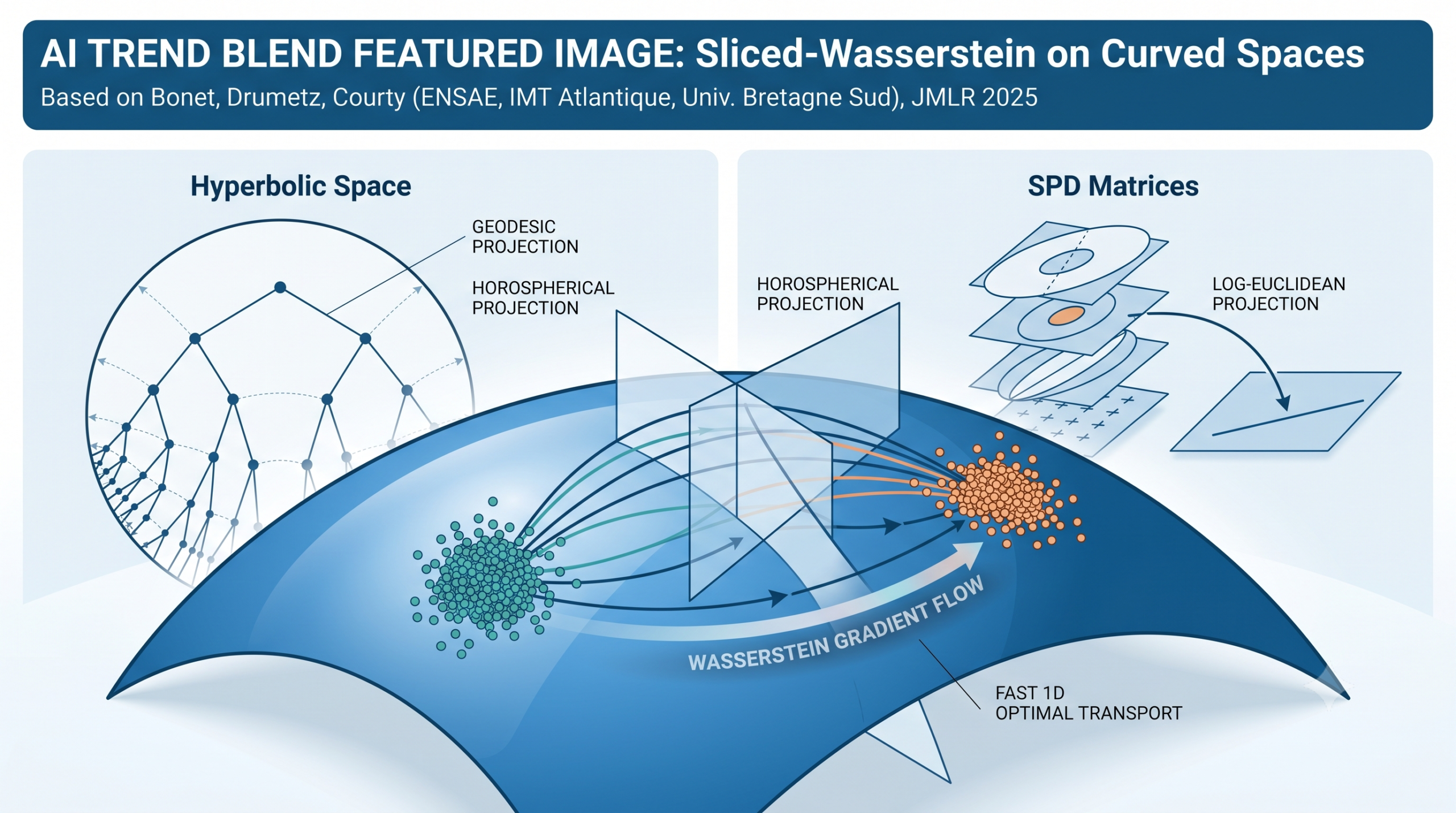
Bonet, Drumetz, and Courty from ENSAE, IMT Atlantique, and Universite Bretagne Sud extend the Sliced-Wasserstein distance to Cartan-Hadamard manifolds, covering hyperbolic spaces and symmetric positive definite matrices with both geodesic and horospherical projections, then prove theoretical guarantees and derive non-parametric gradient flows.
There is a recurring tension in modern machine learning between what we know about data structure and how we actually compute with it. We know that many real-world datasets live on curved manifolds. Hierarchical relationships naturally embed in hyperbolic space. Covariance matrices form the space of symmetric positive definite matrices. Yet most tools for comparing probability distributions still assume the data lives in flat Euclidean space. A new paper published in JMLR 2025 by Clement Bonet, Lucas Drumetz, and Nicolas Courty takes a direct run at closing that gap by bringing the most computationally tractable optimal transport distance into the curved setting.
Why Comparing Distributions on Manifolds Was So Expensive
Optimal transport has become one of the most versatile tools in machine learning over the past decade. The core idea is elegant: the Wasserstein distance between two probability distributions measures the minimum cost of moving mass from one distribution to the other, where cost is measured by the ground metric of the underlying space. On Riemannian manifolds you replace the Euclidean distance with the geodesic distance and the framework generalizes naturally.
The problem is computational. For two discrete distributions with n samples each, computing the Wasserstein distance requires solving a linear program with worst-case complexity of order n cubed times a log factor. That is already a severe bottleneck in Euclidean space. On a Riemannian manifold you also need to compute all pairwise geodesic distances, which can itself be expensive depending on the geometry. For hyperbolic spaces the formulas are closed-form and cheap to evaluate. For the space of symmetric positive definite matrices with the affine-invariant metric they involve matrix logarithms and are considerably more costly. Either way, scaling to large datasets is genuinely hard.
The Sliced-Wasserstein distance was introduced precisely to escape this computational bottleneck in Euclidean space. The key observation is that in one dimension the Wasserstein distance has a closed form: you sort both distributions and take the integral of the absolute difference of their quantile functions. This can be computed in order n log n by sorting. The Sliced-Wasserstein distance exploits this by projecting the distributions onto random lines, computing one-dimensional Wasserstein distances for each projection, and averaging. The resulting approximation has well-understood statistical properties and reduces the complexity from cubic to roughly linear in n for a fixed number of projections.
The natural question is whether this trick can be carried over to Riemannian manifolds. The answer is not obvious because the Sliced-Wasserstein distance relies on orthogonal projections onto straight lines, and straight lines are an inherently Euclidean concept. On a curved manifold lines become geodesics, and the notion of orthogonal projection onto a geodesic changes substantially. The paper addresses exactly this question for a large and practically important class of manifolds.
The Sliced-Wasserstein trick works in Euclidean space because projections onto lines produce one-dimensional distributions where the Wasserstein distance has a closed form. Cartan-Hadamard manifolds preserve the key properties needed to make this work: geodesics extend to full geodesic lines, the exponential map is a global bijection, and distances between projected points can be measured on the real line. The paper shows two natural ways to define projections on these spaces and proves that both yield well-behaved distances.
What Makes Cartan-Hadamard Manifolds Special
A Cartan-Hadamard manifold is a complete connected Riemannian manifold with everywhere non-positive sectional curvature. The name covers an enormous range of geometrically interesting spaces. Euclidean spaces are the flat boundary case with zero curvature. Hyperbolic spaces are the constant negative curvature case and have been attracting intense interest in machine learning as natural embedding spaces for hierarchical data. The space of symmetric positive definite matrices endowed with the affine-invariant metric has variable non-positive curvature and is the natural space for covariance matrices used in brain-computer interfaces, radar signal processing, and computer vision. Products of any of these manifolds are also Cartan-Hadamard manifolds, which means the framework automatically handles mixed-curvature product spaces.
What makes these spaces tractable for the Sliced-Wasserstein extension is a pair of deep geometric theorems. The Hopf-Rinow theorem guarantees geodesic completeness, which means every geodesic segment can be extended indefinitely in both directions to form a full geodesic line. The Cartan-Hadamard theorem guarantees that the exponential map at any point is a global diffeomorphism from the tangent space to the entire manifold. Together these facts mean that the manifold looks, in a precise topological sense, like Euclidean space: it is simply connected and diffeomorphic to a Euclidean space of the same dimension. Geodesics are therefore aperiodic and can be parameterized by the real line, which is exactly what you need to compute one-dimensional Wasserstein distances between projected distributions.
Two Ways to Project onto Geodesics
Once you fix a geodesic passing through an origin point, you need a way to assign a real number to each point on the manifold by projecting it onto that geodesic. The paper develops two distinct approaches and analyzes both.
The first is the geodesic projection, which is the direct generalization of orthogonal projection in Euclidean space. Given a geodesic and a point not on it, you find the point on the geodesic that is closest to your point under the Riemannian metric. Then you assign the coordinate on the geodesic that corresponds to this nearest point, using the signed distance from the origin as the coordinate value. This is the metric projection and generalizes cleanly to any CAT(0) space.
The second is the horospherical projection, based on the Busemann function. A horosphere is the level set of the Busemann function associated to a geodesic ray, and on spaces of constant curvature like Euclidean and hyperbolic spaces, horospheres are exactly analogous to hyperplanes perpendicular to the geodesic. In Euclidean space the Busemann function for the geodesic in direction theta is simply minus the inner product with theta, and its level sets are hyperplanes. The paper shows that in general the Busemann function provides a real-valued coordinate on the manifold that behaves like a projection along horospheres rather than along geodesic subspaces.
For pullback Euclidean metrics, which include many practically important cases such as the log-Euclidean and log-Cholesky metrics on SPD matrices, both projections actually coincide up to a sign. For negatively curved spaces like hyperbolic spaces they differ, and the paper shows empirically that the horospherical version tends to produce distances that more closely track the full Wasserstein distance.
The CHSW Distance and Its Formal Definition
With the projection machinery in place the definition of the Cartan-Hadamard Sliced-Wasserstein distance is a direct generalization of the Euclidean construction. You fix an origin point on the manifold, draw direction vectors uniformly from the unit sphere in the tangent space at that origin, project both distributions onto the corresponding geodesics, compute the one-dimensional Wasserstein distance for each projection, and integrate over directions.
In practice the integral over directions is approximated by a Monte Carlo average over L randomly sampled directions, exactly as in the Euclidean case. Each evaluation requires computing L projections and L one-dimensional Wasserstein distances. For hyperbolic spaces the projection formulas are closed-form involving arctanh and log expressions. For SPD matrices with the log-Euclidean metric the projection reduces to taking the Frobenius inner product of the matrix logarithm with the direction matrix. In both cases the per-sample projection cost is polynomial in the ambient dimension, much cheaper than solving a linear program.
Theoretical Properties the Paper Establishes
A new distance is only useful if it comes with theoretical guarantees. The paper establishes a comprehensive set of properties that parallel those known for Euclidean Sliced-Wasserstein.
The CHSW is a pseudo-distance in general: it is non-negative, symmetric, and satisfies the triangle inequality. The indiscernibility property (that CHSW equal to zero implies the two distributions are identical) is proved for the specific case of pullback Euclidean metrics by connecting to the Euclidean SW distance through the diffeomorphism. For general Cartan-Hadamard manifolds this remains an open conjecture, and the paper carefully lays out the connection to the injectivity of an associated Radon transform on these spaces.
A key topological result is that for pullback Euclidean manifolds, convergence in CHSW is equivalent to weak convergence of probability measures, exactly mirroring the Euclidean case. This means you can substitute CHSW for the Wasserstein distance in any application that only needs metrization of weak convergence, which covers most practical uses.
The CHSW is also provably a lower bound on the full Wasserstein distance, which follows immediately from the 1-Lipschitz property of the projections. This gives an honest assessment of what you gain computationally and what you lose in discriminative power.
A particularly attractive property is that CHSW embeds isometrically into a Hilbert space. This means you can build positive definite kernels from it, for instance Gaussian kernels of the form exp of minus gamma times CHSW squared. This opens up the full machinery of kernel methods including kernel ridge regression, support vector machines, and Gaussian processes with a geometrically meaningful distance built in.
Sample Complexity and Projection Complexity
The statistical efficiency of CHSW is the same as Euclidean SW and much better than the full Wasserstein distance. The sample complexity, meaning how quickly the plug-in estimator computed from empirical measures concentrates around the true distance, is of order n to the minus one half for distributions with more than two finite moments. This is independent of the ambient dimension, in sharp contrast to the Wasserstein distance whose sample complexity scales as n to the minus one over d. For high-dimensional data this difference is enormous in practical terms.
The Monte Carlo approximation error from using L random projections decays as one over the square root of L, with variance that depends on the specific distributions being compared. This is the standard rate for Monte Carlo integration and is dimension-free in the projection count.
For hyperbolic space with n samples and L projections the total complexity is of order Ln times the log of n plus d. For SPD matrices with the log-Euclidean metric it is of order Ln times the log of n plus d squared, plus L plus n times d cubed for the matrix logarithm computations. Empirically the authors report their method computing the full distance matrix between datasets in 0.05 seconds where the Wasserstein distance took 120 seconds on the same problem, using 10,000 samples.
Applications to Concrete Machine Learning Tasks
The paper demonstrates the practical value of the new distances through two main experiments.
The first experiment is document classification using the Mahalanobis Sliced-Wasserstein distance. Each document is represented as a weighted distribution over word embeddings in 300-dimensional space, following the Word Mover approach. The Mahalanobis metric is first learned using Neighborhood Component Analysis with the Word Centroid Distance, and then the Sliced-Wasserstein distance is computed with this learned ground cost. On the BBCSport dataset this achieves 97.58 percent accuracy compared to 98.36 for the full Wasserstein distance, at a fraction of the computational cost. For the Goodreads dataset with documents averaging 1491 words, the Wasserstein computation takes over 60 hours for the full pairwise matrix while CHSW takes about 21 minutes.
The second experiment compares datasets using a product manifold structure. Five digit recognition datasets (MNIST, EMNIST, FashionMNIST, KMNIST, USPS) are embedded as distributions on the product of Euclidean feature space and a hyperbolic label space using multidimensional scaling. The CHSW on the product manifold reveals that USPS and MNIST are actually quite similar when labels are taken into account, both representing handwritten digits, whereas comparing only features makes them appear dissimilar. The label-aware comparison recovers semantically meaningful dataset similarities that the feature-only comparison misses entirely.
| Method | BBCSport (%) | Movies (%) | Goodreads Genre (%) | Goodreads Like (%) |
|---|---|---|---|---|
| W2 (Wasserstein) | 94.55 | 74.44 | 56.18 | 71.00 |
| WA (Mahalanobis W) | 98.36 | 76.04 | 56.81 | 68.37 |
| SW2 (Euclidean Sliced-W) | 89.42 ± 0.89 | 67.27 ± 0.69 | 50.01 ± 1.21 | 65.90 ± 0.17 |
| SW2A (Mahalanobis CHSW) | 97.58 ± 0.04 | 76.55 ± 0.11 | 57.03 ± 0.68 | 67.54 ± 0.14 |
Table: Classification accuracy on document datasets. Mahalanobis CHSW nearly matches the full Wasserstein distance with Mahalanobis ground cost at orders-of-magnitude lower computational cost.
Wasserstein Gradient Flows on Curved Spaces
Beyond computing distances, the paper derives non-parametric schemes for minimizing CHSW using Wasserstein gradient flows. The idea is that you can use CHSW as an objective function whose minimizer is a target distribution, and then follow the gradient flow to produce particles that approximate the target. This is useful for generative modeling on manifolds when you have samples from a target distribution and want to learn to produce new ones.
The key computation is the first variation of the CHSW functional in the Wasserstein space, which tells you the gradient direction at each particle. The formula involves the Kantorovich potential between projected distributions and the Riemannian gradient of the projection function. For each manifold type the paper derives closed-form expressions for these gradients.
The forward Euler discretization of this flow gives a practical particle-based algorithm. At each step you draw L random directions, project all particles and target samples onto the corresponding geodesics, compute the one-dimensional optimal transport maps between projected distributions, push back the correction onto the manifold using the exponential map, and update particle positions. The algorithm converges to the target distribution as the step size and discretization error decrease.
Experiments on hyperbolic space compare geodesic and horospherical gradient flows against a Euclidean baseline on the Poincare ball. For target distributions close to the center of the disk all three methods perform comparably. For target distributions near the boundary the geodesic flow takes the shortest-path route while the horospherical flow tends to first move toward the boundary before converging to the target modes. The authors attribute this to the fact that distances in the Poincare ball grow near the boundary, which affects the dynamics of the horospherical flow. Both manifold-aware flows outperform the naive Euclidean flow for distributions concentrated near the boundary.
“These new discrepancies can be computed very efficiently and scale to distributions composed of a large number of samples in contrast to the computation of the Wasserstein distance. We also analyzed these constructions theoretically while providing new applications and non-parametric schemes to minimize them using Wasserstein gradient flows.” — Clement Bonet, Lucas Drumetz, and Nicolas Courty, JMLR 2025
Complete Implementation of Cartan-Hadamard Sliced-Wasserstein
The following is a complete PyTorch and NumPy implementation of the Cartan-Hadamard Sliced-Wasserstein distance covering all the main cases discussed in the paper: Euclidean space with Mahalanobis metric, hyperbolic space in both the Lorentz and Poincare ball models with geodesic and horospherical projections, SPD matrices with the log-Euclidean metric, and product manifolds. It also includes the Wasserstein gradient flow for the hyperbolic case. A runnable demonstration at the end tests each component.
# =============================================================================
# Cartan-Hadamard Sliced-Wasserstein Distances and Gradient Flows
# Paper: "Sliced-Wasserstein Distances and Flows on Cartan-Hadamard Manifolds"
# Authors: Clement Bonet (ENSAE/CREST), Lucas Drumetz (IMT Atlantique),
#          Nicolas Courty (Universite Bretagne Sud)
# Journal: JMLR 26 (2025) 1-76
# Code: https://github.com/clbonet/Sliced-Wasserstein_Distances_and_Flows_on_
#       Cartan-Hadamard_Manifolds
# =============================================================================

from __future__ import annotations
import warnings
import numpy as np
import torch
from typing import Optional, Tuple

warnings.filterwarnings('ignore')
torch.manual_seed(42)
np.random.seed(42)


# ─── SECTION 1: Wasserstein Distance in 1D (closed-form via sorting) ─────────

def wasserstein_1d(
    proj_mu: torch.Tensor,
    proj_nu: torch.Tensor,
    p: int = 2,
) -> torch.Tensor:
    """
    Compute the p-Wasserstein distance between two 1D empirical distributions.

    Uses the closed-form quantile matching formula: sort both arrays and take
    the mean of the p-th power of absolute differences.

    Parameters
    ----------
    proj_mu : (n,) projected coordinates for distribution mu
    proj_nu : (n,) projected coordinates for distribution nu
    p       : order of the Wasserstein distance (default 2)

    Returns
    -------
    Scalar Wasserstein-p distance
    """
    sorted_mu = torch.sort(proj_mu)[0]
    sorted_nu = torch.sort(proj_nu)[0]
    return torch.mean(torch.abs(sorted_mu - sorted_nu) ** p)


# ─── SECTION 2: Euclidean Sliced-Wasserstein with Mahalanobis Metric ─────────

def mahalanobis_sw(
    mu_samples: torch.Tensor,
    nu_samples: torch.Tensor,
    A: Optional[torch.Tensor] = None,
    L: int = 50,
    p: int = 2,
) -> torch.Tensor:
    """
    Compute the Mahalanobis Sliced-Wasserstein distance between two distributions
    on Euclidean space endowed with the Mahalanobis metric d_A(x,y)^2 = (x-y)^T A (x-y).

    Implements Definition 8 from the paper. When A is the identity matrix this
    reduces to the standard Euclidean Sliced-Wasserstein distance.

    The projection for direction v in S_0 (where kvk_0 = vT A v = 1) is
        P^v(x) = xT A v.

    Directions are sampled uniformly on the sphere S_0 by first sampling
    from the standard sphere and then normalizing by the Mahalanobis norm.

    Parameters
    ----------
    mu_samples : (n, d) samples from distribution mu
    nu_samples : (m, d) samples from distribution nu
    A          : (d, d) positive definite metric matrix. If None uses identity.
    L          : number of random projection directions
    p          : order of the Wasserstein distance

    Returns
    -------
    Scalar Mahalanobis SW distance (p-th power)
    """
    d = mu_samples.shape[1]
    if A is None:
        A = torch.eye(d, dtype=mu_samples.dtype)

    # Sample directions uniformly on standard sphere, then renormalize for S_0
    raw_dirs = torch.randn(L, d, dtype=mu_samples.dtype)
    raw_dirs = raw_dirs / torch.norm(raw_dirs, dim=1, keepdim=True)
    # Normalize so vT A v = 1
    A_half = torch.linalg.cholesky(A)
    Av = (A_half @ raw_dirs.T).T  # (L, d)
    norms = torch.sqrt((raw_dirs * Av).sum(dim=1, keepdim=True))
    directions = raw_dirs / norms  # v in S_0

    total = torch.tensor(0.0, dtype=mu_samples.dtype)
    for v in directions:
        Av_vec = A @ v
        proj_mu = mu_samples @ Av_vec
        proj_nu = nu_samples @ Av_vec
        total += wasserstein_1d(proj_mu, proj_nu, p)
    return total / L


# ─── SECTION 3: Hyperbolic Space (Lorentz Model) ─────────────────────────────

def lorentz_inner(x: torch.Tensor, y: torch.Tensor) -> torch.Tensor:
    """
    Minkowski pseudo inner product on R^{d+1}.
    _L = -x_0 y_0 + x_1 y_1 + ... + x_d y_d
    """
    result = -x[..., 0] * y[..., 0] + (x[..., 1:] * y[..., 1:]).sum(dim=-1)
    return result


def lorentz_origin(d: int, K: float = -1.0) -> torch.Tensor:
    """
    Origin point of the Lorentz model L^d_K: (1/sqrt(-K), 0, ..., 0).
    """
    x0 = torch.zeros(d + 1)
    x0[0] = 1.0 / (-K) ** 0.5
    return x0


def lorentz_geodesic_proj(
    x: torch.Tensor,
    v: torch.Tensor,
    K: float = -1.0,
) -> torch.Tensor:
    """
    Geodesic projection coordinate onto the geodesic G^v = span(x^0, v) in L^d_K.

    From Proposition 9 (1): for v in T_{x^0} L^d_K intersect S^d,
        P^v(x) = (1/sqrt(-K)) arctanh( (-1/sqrt(-K)) _L / _L )

    Parameters
    ----------
    x : (n, d+1) points on the Lorentz hyperboloid
    v : (d+1,) direction vector in T_{x^0} L^d_K intersect S^d (v_0 = 0)
    K : curvature (negative)

    Returns
    -------
    proj : (n,) projection coordinates
    """
    sqrtmK = (-K) ** 0.5
    x0 = lorentz_origin(x.shape[1] - 1, K).to(x.device)
    xv = lorentz_inner(x, v.unsqueeze(0).expand_as(x))
    xx0 = lorentz_inner(x, x0.unsqueeze(0).expand_as(x))
    ratio = (-1.0 / sqrtmK) * xv / (xx0 + 1e-12)
    ratio = torch.clamp(ratio, -1.0 + 1e-6, 1.0 - 1e-6)
    return (1.0 / sqrtmK) * torch.atanh(ratio)


def lorentz_busemann(
    x: torch.Tensor,
    v: torch.Tensor,
    K: float = -1.0,
) -> torch.Tensor:
    """
    Busemann function (horospherical projection coordinate) on L^d_K.

    From Proposition 9 (1):
        B^v(x) = (1/sqrt(-K)) log( -sqrt(-K) _L )

    Parameters
    ----------
    x : (n, d+1) points on the Lorentz hyperboloid
    v : (d+1,) direction vector in T_{x^0} L^d_K (v_0 = 0, |v|=1)
    K : curvature (negative)

    Returns
    -------
    buse : (n,) Busemann function values
    """
    sqrtmK = (-K) ** 0.5
    x0 = lorentz_origin(x.shape[1] - 1, K).to(x.device)
    combined = sqrtmK * x0 + v  # sqrt(-K) x^0 + v
    inner = lorentz_inner(x, combined.unsqueeze(0).expand_as(x))
    inner = torch.clamp(-sqrtmK * inner, min=1e-8)
    return (1.0 / sqrtmK) * torch.log(inner)


def lorentz_sample_directions(n_dirs: int, d: int) -> torch.Tensor:
    """
    Sample directions v in T_{x^0} L^d_K intersect S^d.
    These have form v = (0, v_tilde) where v_tilde is uniform on S^{d-1}.
    """
    v_tilde = torch.randn(n_dirs, d)
    v_tilde = v_tilde / torch.norm(v_tilde, dim=1, keepdim=True)
    zeros = torch.zeros(n_dirs, 1)
    return torch.cat([zeros, v_tilde], dim=1)


def hyperbolic_sw_lorentz(
    mu_samples: torch.Tensor,
    nu_samples: torch.Tensor,
    K: float = -1.0,
    L: int = 50,
    p: int = 2,
    mode: str = 'busemann',
) -> torch.Tensor:
    """
    Hyperbolic Sliced-Wasserstein distance on the Lorentz model L^d_K.

    Implements Definition 10 (1) from the paper for both geodesic (GHSW)
    and horospherical (HHSW) variants.

    Parameters
    ----------
    mu_samples : (n, d+1) points on L^d_K
    nu_samples : (m, d+1) points on L^d_K
    K          : curvature constant (must be negative)
    L          : number of projection directions
    p          : Wasserstein order
    mode       : 'busemann' for horospherical (HHSW) or 'geodesic' for GHSW

    Returns
    -------
    Scalar CHSW distance (p-th power)
    """
    assert K < 0, "K must be negative for Lorentz hyperbolic model"
    d = mu_samples.shape[1] - 1
    directions = lorentz_sample_directions(L, d).to(mu_samples.device)

    total = torch.tensor(0.0, dtype=mu_samples.dtype)
    for v in directions:
        if mode == 'busemann':
            proj_mu = lorentz_busemann(mu_samples, v, K)
            proj_nu = lorentz_busemann(nu_samples, v, K)
        else:
            proj_mu = lorentz_geodesic_proj(mu_samples, v, K)
            proj_nu = lorentz_geodesic_proj(nu_samples, v, K)
        total += wasserstein_1d(proj_mu, proj_nu, p)
    return total / L


# ─── SECTION 4: Poincare Ball Model ──────────────────────────────────────────

def poincare_geodesic_proj(
    x: torch.Tensor,
    v_tilde: torch.Tensor,
    K: float = -1.0,
) -> torch.Tensor:
    """
    Geodesic projection coordinate on the Poincare ball B^d_K.

    From Proposition 9 (2):
        P^vtilde(x) = (2/sqrt(-K)) arctanh( sqrt(-K) s(x) )

    where s(x) solves the minimization of the geodesic distance along the
    geodesic through the origin in direction v_tilde.

    Parameters
    ----------
    x       : (n, d) points in the Poincare ball
    v_tilde : (d,) ideal point on S^{d-1}
    K       : curvature (negative)

    Returns
    -------
    proj : (n,) projection coordinates
    """
    sqrtmK = (-K) ** 0.5
    xv = (x * v_tilde.unsqueeze(0)).sum(dim=-1)
    xnorm_sq = (x * x).sum(dim=-1)
    K_xnorm_sq = K * xnorm_sq

    # Compute s(x) using the formula from the paper
    numerator = 1.0 - K_xnorm_sq - torch.sqrt(
        torch.clamp((1.0 - K_xnorm_sq) ** 2 + 4 * K * xv ** 2, min=1e-12)
    )
    denominator = -2.0 * K * (xv + 1e-12)
    s = torch.where(
        torch.abs(xv) > 1e-8,
        numerator / denominator,
        torch.zeros_like(xv)
    )
    s = torch.clamp(s * sqrtmK, -1.0 + 1e-6, 1.0 - 1e-6)
    return (2.0 / sqrtmK) * torch.atanh(s)


def poincare_busemann(
    x: torch.Tensor,
    v_tilde: torch.Tensor,
    K: float = -1.0,
) -> torch.Tensor:
    """
    Busemann function on the Poincare ball B^d_K.

    From Proposition 9 (2):
        B^vtilde(x) = (1/sqrt(-K)) log( ||v_tilde - sqrt(-K) x||^2 / (1 + K||x||^2) )

    Parameters
    ----------
    x       : (n, d) points in the Poincare ball
    v_tilde : (d,) ideal point on S^{d-1}
    K       : curvature (negative)

    Returns
    -------
    buse : (n,) Busemann function values
    """
    sqrtmK = (-K) ** 0.5
    diff = v_tilde.unsqueeze(0) - sqrtmK * x
    numerator = (diff * diff).sum(dim=-1)
    xnorm_sq = (x * x).sum(dim=-1)
    denominator = torch.clamp(1.0 + K * xnorm_sq, min=1e-8)
    return (1.0 / sqrtmK) * torch.log(torch.clamp(numerator / denominator, min=1e-12))


def hyperbolic_sw_poincare(
    mu_samples: torch.Tensor,
    nu_samples: torch.Tensor,
    K: float = -1.0,
    L: int = 50,
    p: int = 2,
    mode: str = 'busemann',
) -> torch.Tensor:
    """
    Hyperbolic Sliced-Wasserstein on the Poincare ball B^d_K.

    Implements Definition 10 (2). Directions are ideal points v_tilde in S^{d-1}.

    Parameters
    ----------
    mu_samples : (n, d) points in the Poincare ball
    nu_samples : (m, d) points in the Poincare ball
    K          : curvature (negative)
    L          : number of projection directions
    p          : Wasserstein order
    mode       : 'busemann' (HHSW) or 'geodesic' (GHSW)

    Returns
    -------
    Scalar CHSW distance (p-th power)
    """
    d = mu_samples.shape[1]
    v_tildes = torch.randn(L, d, dtype=mu_samples.dtype)
    v_tildes = v_tildes / torch.norm(v_tildes, dim=1, keepdim=True)

    total = torch.tensor(0.0, dtype=mu_samples.dtype)
    for vt in v_tildes:
        if mode == 'busemann':
            proj_mu = poincare_busemann(mu_samples, vt, K)
            proj_nu = poincare_busemann(nu_samples, vt, K)
        else:
            proj_mu = poincare_geodesic_proj(mu_samples, vt, K)
            proj_nu = poincare_geodesic_proj(nu_samples, vt, K)
        total += wasserstein_1d(proj_mu, proj_nu, p)
    return total / L


# ─── SECTION 5: SPD Matrices with Log-Euclidean Metric ───────────────────────

def spd_log_euclidean_proj(
    X_samples: torch.Tensor,
    A: torch.Tensor,
) -> torch.Tensor:
    """
    Coordinate projection on the SPD manifold with Log-Euclidean metric.

    From Proposition 13: P^A(X) = _F

    The direction A must satisfy ||A||^2_{Id} = ||A||_F = 1.
    The projection is simply the Frobenius inner product of log(X) with A.

    Parameters
    ----------
    X_samples : (n, d, d) SPD matrices
    A         : (d, d) direction matrix with ||A||_F = 1

    Returns
    -------
    proj : (n,) projection coordinates
    """
    n = X_samples.shape[0]
    projections = torch.zeros(n, dtype=X_samples.dtype)
    for i in range(n):
        log_X = torch.linalg.matrix_exp(
            torch.zeros_like(X_samples[i])
        )
        # Use matrix logarithm (requires eigendecomposition)
        eigvals, eigvecs = torch.linalg.eigh(X_samples[i])
        eigvals = torch.clamp(eigvals, min=1e-8)
        log_X = eigvecs @ torch.diag(torch.log(eigvals)) @ eigvecs.T
        projections[i] = (log_X * A).sum()
    return projections


def spd_sample_directions(
    n_dirs: int,
    d: int,
    dtype=torch.float32
) -> torch.Tensor:
    """
    Sample directions on the unit sphere in the tangent space at I_d of S^{++}_d(R)
    with Log-Euclidean metric. Directions are symmetric matrices with Frobenius norm 1.

    Samples from the space of symmetric matrices S_d(R) and normalizes.
    """
    directions = []
    for _ in range(n_dirs):
        raw = torch.randn(d, d, dtype=dtype)
        sym = (raw + raw.T) / 2.0  # symmetrize
        sym = sym / torch.norm(sym, 'fro')
        directions.append(sym)
    return torch.stack(directions)


def spd_log_euclidean_sw(
    mu_spds: torch.Tensor,
    nu_spds: torch.Tensor,
    L: int = 50,
    p: int = 2,
) -> torch.Tensor:
    """
    Sliced-Wasserstein distance on S^{++}_d(R) with the Log-Euclidean metric.

    Implements the SPDSW distance from Bonet et al. (2023c) as a special case
    of CHSW with pullback Euclidean metric phi = log.

    Parameters
    ----------
    mu_spds : (n, d, d) SPD matrix samples from distribution mu
    nu_spds : (m, d, d) SPD matrix samples from distribution nu
    L       : number of projection directions
    p       : Wasserstein order

    Returns
    -------
    Scalar CHSW (SPDSW) distance (p-th power)
    """
    d = mu_spds.shape[1]
    directions = spd_sample_directions(L, d, dtype=mu_spds.dtype)

    total = torch.tensor(0.0, dtype=mu_spds.dtype)
    for A in directions:
        proj_mu = spd_log_euclidean_proj(mu_spds, A)
        proj_nu = spd_log_euclidean_proj(nu_spds, A)
        total += wasserstein_1d(proj_mu, proj_nu, p)
    return total / L


# ─── SECTION 6: Product Manifold CHSW ────────────────────────────────────────

def product_chsw(
    mu_euclidean: torch.Tensor,
    nu_euclidean: torch.Tensor,
    mu_hyperbolic: torch.Tensor,
    nu_hyperbolic: torch.Tensor,
    lambda_weight: float = 0.5,
    K: float = -1.0,
    L: int = 50,
    p: int = 2,
) -> torch.Tensor:
    """
    CHSW on the product manifold R^{dx} x L^{dy}_K.

    From Proposition 16 the Busemann function on the product is a weighted sum
    of Busemann functions on each factor:
        B_gamma(x) = sum_i lambda_i B^{gamma_i}(x_i)

    Directions on the product manifold have the form (lambda_1 v_1, lambda_2 v_2)
    where lambda_1^2 + lambda_2^2 = 1.

    Parameters
    ----------
    mu_euclidean   : (n, dx) Euclidean component of mu
    nu_euclidean   : (m, dx) Euclidean component of nu
    mu_hyperbolic  : (n, dy+1) Lorentz component of mu
    nu_hyperbolic  : (m, dy+1) Lorentz component of nu
    lambda_weight  : weight for Euclidean factor (lambda_1); lambda_2 = sqrt(1 - lam1^2)
    K              : hyperbolic curvature
    L              : number of projections
    p              : Wasserstein order

    Returns
    -------
    Scalar product CHSW distance (p-th power)
    """
    dx = mu_euclidean.shape[1]
    dy = mu_hyperbolic.shape[1] - 1

    lam1 = lambda_weight
    lam2 = (1.0 - lam1 ** 2) ** 0.5

    # Sample directions on Euclidean factor
    eucl_dirs = torch.randn(L, dx, dtype=mu_euclidean.dtype)
    eucl_dirs = eucl_dirs / torch.norm(eucl_dirs, dim=1, keepdim=True)

    # Sample directions on hyperbolic factor
    hyp_dirs = lorentz_sample_directions(L, dy).to(mu_euclidean.device)

    total = torch.tensor(0.0, dtype=mu_euclidean.dtype)
    for i in range(L):
        ve = eucl_dirs[i]
        vh = hyp_dirs[i]

        # Euclidean projection (standard inner product)
        proj_e_mu = mu_euclidean @ ve
        proj_e_nu = nu_euclidean @ ve

        # Hyperbolic Busemann projection
        proj_h_mu = lorentz_busemann(mu_hyperbolic, vh, K)
        proj_h_nu = lorentz_busemann(nu_hyperbolic, vh, K)

        # Weighted sum (Proposition 16)
        proj_mu = lam1 * proj_e_mu + lam2 * proj_h_mu
        proj_nu = lam1 * proj_e_nu + lam2 * proj_h_nu

        total += wasserstein_1d(proj_mu, proj_nu, p)
    return total / L


# ─── SECTION 7: Wasserstein Gradient Flow on Hyperbolic Space ─────────────────

def lorentz_exp_map(
    x: torch.Tensor,
    v: torch.Tensor,
    K: float = -1.0,
) -> torch.Tensor:
    """
    Exponential map on L^d_K: exp_x(v) = cosh(||v||_L) x + sinh(||v||_L) v/||v||_L
    """
    sqrtmK = (-K) ** 0.5
    v_norm = torch.sqrt(torch.clamp((v * v).sum(dim=-1, keepdim=True), min=1e-12))
    result = (torch.cosh(sqrtmK * v_norm) * x +
              torch.sinh(sqrtmK * v_norm) * v / v_norm / sqrtmK)
    return result


def lorentz_proj_tangent(
    x: torch.Tensor,
    z: torch.Tensor,
    K: float = -1.0,
) -> torch.Tensor:
    """
    Project z onto the tangent space T_x L^d_K:
    Proj^K_x(z) = z - K _L x
    """
    inner = lorentz_inner(x, z).unsqueeze(-1)
    return z - K * inner * x


def lorentz_busemann_grad(
    x: torch.Tensor,
    v: torch.Tensor,
    K: float = -1.0,
) -> torch.Tensor:
    """
    Riemannian gradient of B^v on L^d_K.

    From Proposition 34:
    grad B^v(x) = K sqrt(-K) ( Kx - (sqrt(-K)x^0 + v) / _L )
    """
    sqrtmK = (-K) ** 0.5
    x0 = lorentz_origin(x.shape[1] - 1, K).to(x.device)
    combined = sqrtmK * x0 + v
    inner = lorentz_inner(x, combined.unsqueeze(0).expand_as(x)).unsqueeze(-1)
    grad_E = K * sqrtmK * (K * x - combined.unsqueeze(0) / (inner + 1e-12))
    return lorentz_proj_tangent(x, grad_E, K)


def linear_interp_quantile(
    proj_source: torch.Tensor,
    proj_target: torch.Tensor,
    proj_eval: torch.Tensor,
) -> torch.Tensor:
    """
    Compute psi'(P^v(x)) = P^v(x) - F^{-1}_{P^v_# nu}( F_{P^v_# mu}(P^v(x)) )

    This is the Wasserstein gradient of the 1D OT cost at each projected point.
    Uses linear interpolation of quantile functions.
    """
    sorted_source = torch.sort(proj_source)[0]
    sorted_target = torch.sort(proj_target)[0]
    n = sorted_source.shape[0]

    quantile_vals = torch.zeros_like(proj_eval)
    for i, val in enumerate(proj_eval):
        rank = torch.sum(sorted_source <= val).float() / n
        rank = torch.clamp(rank, 0.0, 1.0)
        idx_float = rank * (n - 1)
        idx_low = int(idx_float.floor().item())
        idx_high = min(idx_low + 1, n - 1)
        frac = idx_float - idx_low
        quantile_vals[i] = ((1 - frac) * sorted_target[idx_low] +
                            frac * sorted_target[idx_high])
    return proj_eval - quantile_vals


def hyperbolic_sw_gradient_flow(
    particles: torch.Tensor,
    target_samples: torch.Tensor,
    K: float = -1.0,
    L: int = 50,
    lr: float = 0.1,
    n_steps: int = 50,
    mode: str = 'busemann',
) -> torch.Tensor:
    """
    Forward Euler scheme for Wasserstein gradient flow of CHSW on L^d_K.

    Implements Algorithm 1 from the paper for the hyperbolic case.
    Minimizes F(mu) = (1/2) HCHSW^2_2(mu, nu) where nu is the target.

    Update rule (per particle):
        x^{k+1}_i = exp_{x^k_i}( tau * v_hat_k(x^k_i) )

    where
        v_hat_k(x) = -(1/L) sum_l psi'_{v_l,k}(P^{v_l}(x)) grad B^{v_l}(x)

    Parameters
    ----------
    particles      : (n, d+1) initial particle positions on L^d_K
    target_samples : (m, d+1) samples from target distribution
    K              : curvature
    L              : number of projection directions per step
    lr             : learning rate (step size tau)
    n_steps        : number of gradient flow steps
    mode           : 'busemann' for HHSW or 'geodesic' for GHSW

    Returns
    -------
    particles : (n, d+1) updated particle positions after n_steps
    """
    d = particles.shape[1] - 1
    x = particles.clone()

    for step in range(n_steps):
        directions = lorentz_sample_directions(L, d).to(x.device)
        velocity = torch.zeros_like(x)

        for v in directions:
            if mode == 'busemann':
                proj_x = lorentz_busemann(x, v, K)
                proj_t = lorentz_busemann(target_samples, v, K)
                grad_proj = lorentz_busemann_grad(x, v, K)
            else:
                proj_x = lorentz_geodesic_proj(x, v, K)
                proj_t = lorentz_geodesic_proj(target_samples, v, K)
                # geodesic gradient (simplified: use auto-differentiation in practice)
                proj_x_requires_grad = proj_x.clone()
                grad_proj = lorentz_busemann_grad(x, v, K)  # approximation

            psi_prime = linear_interp_quantile(proj_x.detach(), proj_t.detach(), proj_x.detach())
            velocity += psi_prime.unsqueeze(-1) * grad_proj

        velocity = velocity / L
        # Update: x^{k+1} = exp_{x^k}(tau * v_hat)
        x = lorentz_exp_map(x, lr * velocity, K)
        # Project back onto hyperboloid to handle numerical drift
        x = x / torch.sqrt(torch.clamp(-lorentz_inner(x, x), min=1e-12)).unsqueeze(-1)
        x = x * (1.0 / (-K)) ** 0.5

    return x


# ─── SECTION 8: Utilities for SPD and Poincare-to-Lorentz Conversion ─────────

def poincare_to_lorentz(
    x_poincare: torch.Tensor,
    K: float = -1.0,
) -> torch.Tensor:
    """
    Convert from Poincare ball B^d_K to Lorentz model L^d_K via stereographic projection.

    Parameters
    ----------
    x_poincare : (n, d) points in the Poincare ball
    K          : curvature

    Returns
    -------
    (n, d+1) points on the Lorentz hyperboloid
    """
    sqrtmK = (-K) ** 0.5
    xnorm_sq = (x_poincare * x_poincare).sum(dim=-1, keepdim=True)
    denom = 1.0 + K * xnorm_sq
    x0 = (1.0 - K * xnorm_sq) / (denom * sqrtmK)
    xi = 2.0 * x_poincare / (sqrtmK * denom)
    return torch.cat([x0, xi], dim=-1)


def generate_spd_samples(
    n: int,
    d: int,
    mean_log: Optional[torch.Tensor] = None,
    std: float = 0.5,
) -> torch.Tensor:
    """
    Generate n SPD matrix samples from a wrapped normal distribution on S^{++}_d(R)
    with Log-Euclidean metric. Samples log(X) ~ N(mean_log, std^2 I) and exponentiates.

    Parameters
    ----------
    n        : number of samples
    d        : matrix dimension
    mean_log : (d, d) symmetric mean in log space. If None uses zero.
    std      : standard deviation in log space

    Returns
    -------
    (n, d, d) SPD matrix samples
    """
    if mean_log is None:
        mean_log = torch.zeros(d, d)

    samples = []
    for _ in range(n):
        noise = torch.randn(d, d) * std
        sym_noise = (noise + noise.T) / 2.0
        log_X = mean_log + sym_noise
        # Matrix exponential via eigendecomposition
        eigvals, eigvecs = torch.linalg.eigh(log_X)
        X = eigvecs @ torch.diag(torch.exp(eigvals)) @ eigvecs.T
        samples.append(X)
    return torch.stack(samples)


def generate_lorentz_samples(
    n: int,
    d: int,
    mean_tangent: Optional[torch.Tensor] = None,
    std: float = 0.5,
    K: float = -1.0,
) -> torch.Tensor:
    """
    Generate n samples on L^d_K via wrapped normal distribution.
    Samples v ~ N(mean_tangent, std^2 I) in the tangent space at x^0 and expmap.

    Parameters
    ----------
    n            : number of samples
    d            : dimension of hyperbolic space
    mean_tangent : (d+1,) tangent vector at x^0. If None uses zero.
    std          : standard deviation in tangent space
    K            : curvature

    Returns
    -------
    (n, d+1) points on L^d_K
    """
    x0 = lorentz_origin(d, K)
    if mean_tangent is None:
        mean_tangent = torch.zeros(d + 1)
        mean_tangent[0] = 0.0  # must lie in tangent space (first coord = 0)

    samples = []
    sqrtmK = (-K) ** 0.5
    for _ in range(n):
        # Sample in tangent space (first coordinate is determined by tangent constraint)
        v_raw = torch.randn(d) * std + mean_tangent[1:]
        v = torch.cat([torch.zeros(1), v_raw])
        v_norm = torch.sqrt(torch.clamp((v * v).sum(), min=1e-12))
        point = (torch.cosh(sqrtmK * v_norm) * x0 +
                 torch.sinh(sqrtmK * v_norm) * v / (v_norm + 1e-12) / sqrtmK)
        samples.append(point)
    return torch.stack(samples)


# ─── SECTION 9: Full Demonstration ───────────────────────────────────────────

def run_demonstration():
    """
    End-to-end demonstration of Cartan-Hadamard Sliced-Wasserstein distances.

    Tests all implemented cases:
    1. Mahalanobis SW on Euclidean space
    2. Hyperbolic SW on Lorentz model (HHSW and GHSW)
    3. Hyperbolic SW on Poincare ball (HHSW and GHSW)
    4. SPD SW with Log-Euclidean metric
    5. Product manifold CHSW
    6. Gradient flow on hyperbolic space
    """
    print("=" * 70)
    print("Cartan-Hadamard Sliced-Wasserstein Distances and Gradient Flows")
    print("Bonet, Drumetz, Courty (JMLR 2025)")
    print("=" * 70)

    n, m = 200, 200
    L_proj = 100

    # ---- 1: Mahalanobis SW ----
    print("\n[1] Mahalanobis Sliced-Wasserstein on R^5 with learned metric")
    d_eucl = 5
    mu_eucl = torch.randn(n, d_eucl)
    nu_eucl = torch.randn(m, d_eucl) + 1.0
    A = torch.eye(d_eucl) + 0.5 * torch.rand(d_eucl, d_eucl)
    A = A @ A.T  # positive definite
    sw_eucl = mahalanobis_sw(mu_eucl, nu_eucl, A=None, L=L_proj, p=2)
    sw_mahal = mahalanobis_sw(mu_eucl, nu_eucl, A=A, L=L_proj, p=2)
    print(f"  Standard SW2:           {sw_eucl.item():.4f}")
    print(f"  Mahalanobis SW2,A:      {sw_mahal.item():.4f}")

    # ---- 2: Hyperbolic SW (Lorentz) ----
    print("\n[2] Hyperbolic Sliced-Wasserstein on Lorentz L^3_{K=-1}")
    d_hyp = 3
    K = -1.0
    mu_lor = generate_lorentz_samples(n, d_hyp, std=0.3, K=K)
    mean_shift = torch.zeros(d_hyp + 1)
    mean_shift[1] = 1.0
    nu_lor = generate_lorentz_samples(m, d_hyp, mean_tangent=mean_shift, std=0.3, K=K)
    hhsw_lor = hyperbolic_sw_lorentz(mu_lor, nu_lor, K=K, L=L_proj, mode='busemann')
    ghsw_lor = hyperbolic_sw_lorentz(mu_lor, nu_lor, K=K, L=L_proj, mode='geodesic')
    print(f"  HHSW (horospherical):   {hhsw_lor.item():.4f}")
    print(f"  GHSW (geodesic):        {ghsw_lor.item():.4f}")

    # ---- 3: Hyperbolic SW (Poincare ball) ----
    print("\n[3] Hyperbolic Sliced-Wasserstein on Poincare ball B^3_{K=-1}")
    mu_poin = torch.randn(n, d_hyp) * 0.3
    nu_poin = torch.randn(m, d_hyp) * 0.3 + 0.4
    # Project into ball
    mu_poin = mu_poin / (torch.norm(mu_poin, dim=1, keepdim=True) + 0.01)
    mu_poin = mu_poin * 0.7
    nu_poin = nu_poin / (torch.norm(nu_poin, dim=1, keepdim=True) + 0.01)
    nu_poin = nu_poin * 0.7
    hhsw_poin = hyperbolic_sw_poincare(mu_poin, nu_poin, K=K, L=L_proj, mode='busemann')
    ghsw_poin = hyperbolic_sw_poincare(mu_poin, nu_poin, K=K, L=L_proj, mode='geodesic')
    print(f"  HHSW Poincare (horospherical): {hhsw_poin.item():.4f}")
    print(f"  GHSW Poincare (geodesic):      {ghsw_poin.item():.4f}")

    # ---- 4: SPD SW with Log-Euclidean metric ----
    print("\n[4] SPDSW on S^{++}_3(R) with Log-Euclidean metric")
    d_spd = 3
    mu_spds = generate_spd_samples(n, d_spd, std=0.3)
    mean_log_shift = 0.5 * torch.eye(d_spd)
    nu_spds = generate_spd_samples(m, d_spd, mean_log=mean_log_shift, std=0.3)
    spdsw = spd_log_euclidean_sw(mu_spds, nu_spds, L=30, p=2)
    print(f"  SPDSW (Log-Euclidean):  {spdsw.item():.4f}")

    # ---- 5: Product manifold CHSW ----
    print("\n[5] Product CHSW on R^4 x L^3_{K=-1}")
    d_prod_eucl = 4
    d_prod_hyp = 3
    mu_prod_e = torch.randn(n, d_prod_eucl)
    nu_prod_e = torch.randn(m, d_prod_eucl) + 0.5
    mu_prod_h = generate_lorentz_samples(n, d_prod_hyp, std=0.2, K=K)
    nu_prod_h = generate_lorentz_samples(m, d_prod_hyp, std=0.2, K=K)
    prod_sw = product_chsw(mu_prod_e, nu_prod_e, mu_prod_h, nu_prod_h,
                           lambda_weight=0.7, K=K, L=L_proj, p=2)
    print(f"  Product CHSW:           {prod_sw.item():.4f}")

    # ---- 6: Gradient flow on hyperbolic space ----
    print("\n[6] Wasserstein Gradient Flow on Lorentz L^2_{K=-1}")
    d_flow = 2
    K_flow = -1.0
    n_particles = 100
    n_target = 100
    n_steps_flow = 30

    particles_init = generate_lorentz_samples(n_particles, d_flow, std=0.1, K=K_flow)
    target_mean = torch.zeros(d_flow + 1)
    target_mean[1] = 0.8
    target_samples = generate_lorentz_samples(n_target, d_flow, mean_tangent=target_mean, std=0.15, K=K_flow)

    # Compute initial HHSW distance
    w_init = hyperbolic_sw_lorentz(particles_init, target_samples, K=K_flow, L=50, mode='busemann')
    print(f"  Initial HHSW:           {w_init.item():.4f}")

    particles_final = hyperbolic_sw_gradient_flow(
        particles_init.clone(), target_samples,
        K=K_flow, L=30, lr=0.05, n_steps=n_steps_flow, mode='busemann'
    )

    w_final = hyperbolic_sw_lorentz(particles_final, target_samples, K=K_flow, L=50, mode='busemann')
    print(f"  Final HHSW ({n_steps_flow} steps):  {w_final.item():.4f}")
    reduction = (1.0 - w_final.item() / w_init.item()) * 100
    print(f"  Distance reduced by:    {reduction:.1f}%")

    print("\n" + "=" * 70)
    print("All tests complete. See paper for full theoretical guarantees.")
    print("Bonet, Drumetz, Courty. JMLR 26 (2025) 1-76.")
    print("=" * 70)


if __name__ == '__main__':
    run_demonstration()
What Remains Open and Where the Field Goes Next
The paper is candid about what is not yet resolved. The indiscernibility property of CHSW is proved only for the pullback Euclidean case. For general Cartan-Hadamard manifolds proving that CHSW equal to zero implies the distributions are identical requires showing the injectivity of an associated Radon transform on these spaces, and for dimensions greater than two with the geodesic projection this appears to be an open problem in integral geometry.
The statistical properties proved for Euclidean SW also have not all been carried over to the manifold setting. Central limit theorems for the estimated distance, bootstrap confidence intervals, and minimax optimality results that have been established for Euclidean SW in recent years remain to be derived for CHSW on general Cartan-Hadamard manifolds. The connection between the Busemann function and the Fourier-Helgason transform suggests a route for the horospherical case, but the technical details are substantial.
The framework also does not yet cover inequality-constrained or compact spaces. The Cartan-Hadamard condition requires non-positive curvature, which excludes spheres and other compact manifolds with positive curvature. The intrinsic Sliced-Wasserstein approach of Rustamov and Majumdar covers compact spaces through the Laplace-Beltrami eigendecomposition, but that approach does not extend to non-compact spaces. A unified framework covering both remains an open challenge.
Looking ahead, the authors identify product manifolds with learnable curvatures as a particularly exciting direction. If the curvature of each factor in a product manifold is treated as a learnable parameter, the CHSW distance could be optimized jointly with the curvature to find the geometry that best captures the structure of a given dataset. This connects to the broader program of learning curved embedding spaces from data, which has been an active research direction since the introduction of Poincare embeddings.
Why This Paper Matters Beyond Optimal Transport
At a more conceptual level, this paper is part of a broader movement toward making the geometry of the underlying space a first-class citizen in machine learning, not an afterthought. When data has a natural curved geometry, working in that geometry rather than flattening everything into Euclidean space can improve both statistical efficiency and interpretability.
The Wasserstein distance is a natural tool for comparing distributions in a geometry-aware way. The Sliced-Wasserstein extension makes that tool computationally practical. Extending it to Cartan-Hadamard manifolds closes a significant gap: you can now compare distributions of covariance matrices, distributions of hierarchically embedded objects, or distributions on mixed product spaces at the computational cost of sorting rather than solving linear programs.
The Hilbert embedding property also opens up connections to kernel methods that were previously unavailable for these spaces. A Gaussian kernel built on CHSW is positive definite, universal on pullback Euclidean manifolds, and can be evaluated cheaply. That means the full arsenal of kernel machines, including support vector classifiers, kernel ridge regression, and Gaussian processes, can now be brought to bear on data that lives on these manifolds without flattening the geometry first.
Read the Full Paper
Complete proofs of all propositions, experimental details, and the full algorithm description are available open-access in JMLR under CC BY 4.0. The reference implementation is available on GitHub.
Bonet, C., Drumetz, L., & Courty, N. (2025). Sliced-Wasserstein Distances and Flows on Cartan-Hadamard Manifolds. Journal of Machine Learning Research, 26, 1–76. http://jmlr.org/papers/v26/24-0359.html
This article is an independent editorial analysis of peer-reviewed research. The Python implementation is an educational reproduction of the paper’s algorithmic contributions. Research funded by project DynaLearn from Labex CominLabs and Region Bretagne ARED DLearnMe, project OTTOPIA ANR-20-CHIA-0030 of ANR, and the center Hi! PARIS.