Key Points
- Expected Improvement (EI) is designed for simple regret (finding the best final answer) and performs poorly when the goal is cumulative regret (overall performance across all iterations).
- The EIC algorithm adds an evaluation cost gate to each iteration: a new point is sampled only if its EI value exceeds the expected loss from sampling it, scaled by the remaining budget.
- EIC achieves a high-probability regret bound of \(O(\sqrt{N \gamma_N (\log N)^{1/2}})\), matching GP-TS and beating prior EI-based bounds by a factor of \(\sqrt{\gamma_N \log N}\).
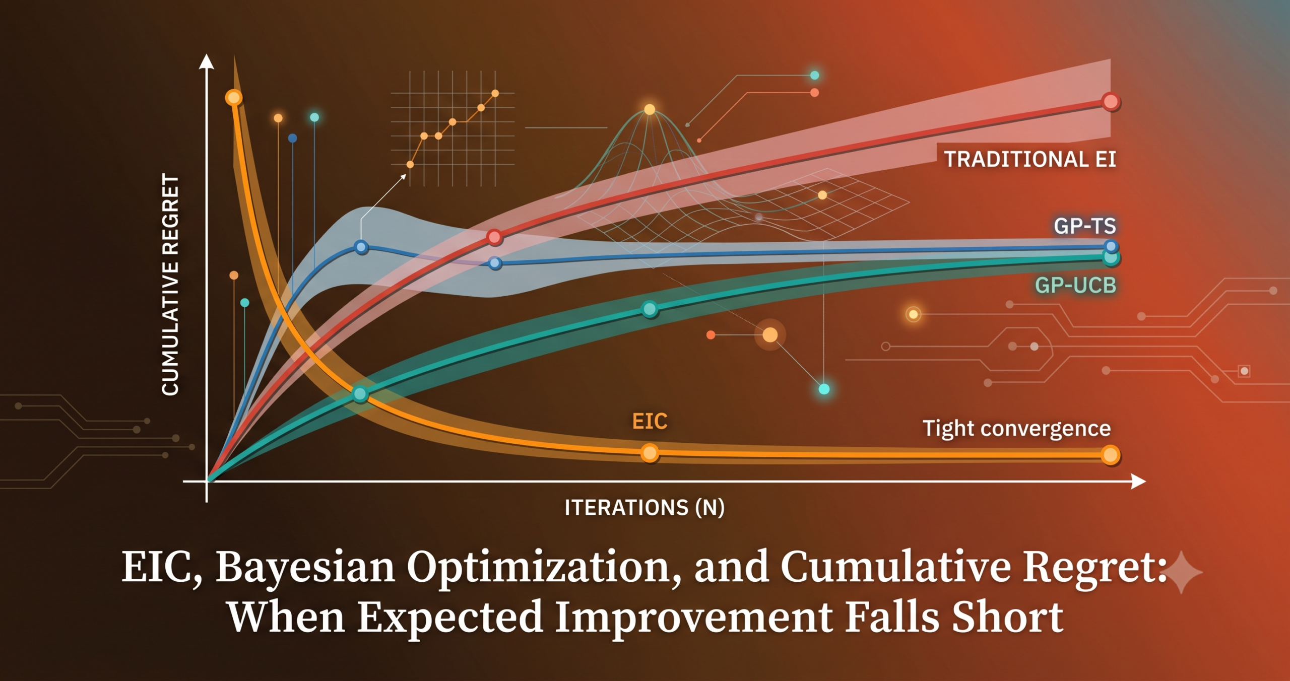
- On six synthetic benchmarks and a cancer-classification hyperparameter tuning task, EIC matches or beats GP-UCB in cumulative regret while maintaining the intuitive EI framework practitioners already understand.
- The evaluation cost has a natural effect over time — it becomes stricter as the budget shrinks, nudging the algorithm from exploration toward exploitation automatically.
- The key lemma (Lemma 2) is tight and shows exactly why the cost gate enables the tighter bound that was previously unavailable to EI.
The gap between what EI optimizes and what pipelines actually need
Expected Improvement has a lot going for it. It has a closed-form expression, it naturally trades off exploration and exploitation, and decades of practitioners have found that it just works. Jones, Schonlau, and Welch popularized it in 1998, and it has been a benchmark acquisition function ever since. The catch is that EI was designed around a specific objective — find the single best point at the end of the experiment. Theoretically, that is called simple regret minimization.
Many real pipelines care about something different. If you are tuning a recommendation system that runs continuously, every intermediate configuration affects real users. The same is true of clinical trial design, where each patient receives the therapy chosen by your current model. In these settings you want the total accumulated quality of all evaluations to be high, not just the final one. That is cumulative regret minimization, and it is a genuinely harder problem because every single iteration counts.
The theoretical gap has been visible for a while. Srinivas et al. (2010) showed that GP-UCB achieves a cumulative regret bound of \(O(\sqrt{N \gamma_N} (\log N)^{3/2})\), later tightened by Chowdhury and Gopalan (2017) to \(O(\sqrt{N \gamma_N})\) for GP-UCB and \(O(\sqrt{N \gamma_N} (\log N)^{1/2})\) for GP-TS. The best EI-based bounds available before this paper were substantially worse. Wang and De Freitas (2014) got \(O(\sqrt{N} \gamma_N^{3/2} \log N)\). Nguyen et al. (2017) improved that to \(O(\sqrt{N} \gamma_N (\log N)^{3/2})\), but their bound depended on a hand-tuned constant that blew up in the limit. The gap was not cosmetic — it reflected something genuinely different about how EI explores.
The paper by Shouri Hu, Haowei Wang, Zhongxiang Dai, Bryan Low, and Szu Hui Ng, published in JMLR 26 in 2025, asks a pointed question — can EI be adapted to close this gap without abandoning the EI framework entirely? The answer is yes, and the mechanism is elegantly simple once you see it. You can read the full paper at JMLR here.
What EI gets wrong under cumulative regret
The acquisition function of EI at iteration \(n\) is:
Here \(\xi_n\) is the incumbent value (some estimate of the current best), \(\mathbb{E}_n\) is the expectation under the current GP posterior, and \((z)^+ = \max(0, z)\). This quantity is the expected gain from sampling \(x\) over the current best. It only looks at the upside.
That is fine when you report only the final answer. If you sample a bad point on iteration 47, it does not matter — you ignore it and report your best at the end. But under cumulative regret, that bad point on iteration 47 goes into your running total and hurts you. EI has no mechanism to avoid that cost because it never looks at the downside of sampling a point.
The second issue is the incumbent. In noisy settings, you cannot observe true function values. The natural choice — the best noisy observation so far — is unstable because noise can make a bad point look good on one run. Wang and De Freitas (2014) suggested using the maximum of the posterior mean over the whole domain, which is stable but computationally expensive and introduces an extra layer of uncertainty. The EIC paper takes a middle path: use the maximum posterior mean at already-observed locations only.
This is stable, avoids a domain-wide optimization step, and — as Lemma 4 in the paper shows — plays nicely with the rest of the regret proof. The signal variance parameter \(\omega_n\) is also set as a scheduled sequence rather than a fixed hyperparameter, with the form \(\omega_n = c_0 \sqrt{\gamma_n + 1 + \log(1/\delta)}\), where \(\gamma_n\) is the maximum information gain and \(\delta\) controls the failure probability. This is what allows the exploration rate to grow appropriately with the information geometry of the problem.
The evaluation cost — why it works
The central contribution of EIC is the evaluation cost function \(L_n(x)\):
The numerator is the expected loss from sampling \(x\) when it turns out to be worse than the incumbent. The denominator is the number of remaining iterations. A new point is sampled only if \(\alpha_n^{\text{EI}}(x) \ge L_n(x)\) for at least one \(x\) in the domain. When no point meets that condition, the algorithm resamples the previously-observed location with the best posterior mean.
The intuition the authors provide is worth sitting with. Suppose at iteration \(n\) you stop exploring and just keep resampling the current best point for all remaining \(N – n\) iterations. Your remaining cumulative regret would be \((N-n)(f(x^*) – \xi_n)\). Now suppose instead you try one new point \(x_{n+1}\) and then decide what to do. If that new point beats the incumbent (expected gain \(\alpha_n^{\text{EI}}(x_{n+1})\)), you can harvest that gain over all \((N-n)\) remaining iterations by sticking with it. If it does not beat the incumbent, you lose the difference once — in iteration \(n+1\) — and then switch back. So \(x_{n+1}\) is worth sampling if and only if:
Divide both sides by \((N-n)\) and you recover exactly the condition \(\alpha_n^{\text{EI}}(x) \ge L_n(x)\). The evaluation cost is not an arbitrary regularizer — it emerges directly from a principled cost-benefit analysis over the remaining horizon.
The EIC algorithm from first principles
Before the main loop begins, EIC runs a structured initialization. The domain \([0,1]^d\) is divided into \(M^d\) equal hypercubes, and one point is placed at the centre of each. The parameter \(M\) is set to \(cN^{1/2d}\) for a constant \(c\), giving \(n_0 = c^d N^{1/2}\) initial points. The purpose is to ensure the GP posterior variance is uniformly controlled across the domain before adaptive sampling begins. As the paper notes, an ill-chosen initial design can cause BO algorithms to fail entirely, and this grid-centred scheme ties the initialization budget directly to the total budget \(N\).
The main loop then proceeds as follows. At each iteration \(n\), the GP posterior is updated, the set \(B_n = \{x : \alpha_n^{\text{EI}}(x) \ge L_n(x)\}\) is identified, and if \(B_n\) is non-empty, the point with the largest EI value in \(B_n\) is sampled. If \(B_n\) is empty, the algorithm resamples the observed point with the highest posterior mean. The selected point receives exactly one function evaluation. This is Algorithm 1 in the paper and it is clean enough to implement in a few dozen lines on top of any existing BO library.
The regret bound and what makes it tick
Under standard regularity conditions (the objective function belongs to the RKHS associated with the GP kernel, the kernel is isotropic and bounded, and the noise is sub-Gaussian), Theorem 1 of the paper establishes that with probability at least \(1 – \delta\):
Here \(\gamma_N\) is the maximum information gain, the maximum mutual information between any \(N\) sampled function values and their noisy observations. This quantity depends on the kernel and grows slowly — polylogarithmically for the squared exponential kernel and as a polynomial of \(N\) for the Matérn kernel. Corollary 1 of the paper spells out the implications for each kernel.
| Algorithm | Regret bound (high probability) | Notes |
|---|---|---|
| GP-UCB (Chowdhury and Gopalan 2017) | \(O(\sqrt{N \gamma_N})\) | Tightest known, frequentist |
| GP-TS (Chowdhury and Gopalan 2017) | \(O(\sqrt{N \gamma_N} (\log N)^{1/2})\) | Bayesian sampling |
| EIC (Hu et al. 2025) | \(O(\sqrt{N \gamma_N} (\log N)^{1/2})\) | First EI-based bound to match GP-TS |
| EI — Nguyen et al. (2017) | \(O(\sqrt{N} \gamma_N (\log N)^{3/2})\) | Constant blows up as threshold goes to zero |
| EI — Wang and De Freitas (2014) | \(O(\sqrt{N} \gamma_N^{3/2} \log N)\) | Extra \(\gamma_N^{1/2}\) factor |
The improvement over Wang and De Freitas (2014) is a factor of roughly \(\sqrt{\gamma_N \log N}\). For the squared exponential kernel, \(\gamma_N\) is polylogarithmic, so the practical difference may seem modest. For the Matérn kernel in moderate dimensions it can be substantial. The Corollary 1 bounds for the Matérn kernel are \(O(N^{(2\nu+3d)/(4\nu+2d)} (\log N)^{(6\nu+d)/(4\nu+2d)})\), which approach the lower bounds of Scarlett et al. (2018) as the smoothness \(\nu\) grows.
The proof structure is worth understanding at a high level. The regret at each iteration decomposes into two terms. Term [I] is the gap between the global optimum and the current incumbent, bounded using a ratio of EI values at the new point and the optimum. Term [II] is the gap between the incumbent and the newly sampled point. This is where the evaluation cost gate does its work. Lemma 2 — the central technical contribution of the paper — shows that whenever a point passes the cost gate, the standardized quantity \(z_n(x) = (\mu_n(x) – \xi_n) / \sigma_n(x)\) must be no smaller than \(-\omega_n \sqrt{2 \log(N-n)}\). Without the cost gate, this lower bound is unavailable, and Term [II] cannot be controlled as tightly.
What the experiments actually show
The authors ran 100 independent trials on six synthetic test functions spanning two to six dimensions, plus a real-world neural network hyperparameter tuning task. Each experiment compared EIC, standard EI, EI-Nguyen (the Nguyen et al. 2017 variant with threshold \(\kappa = 10^{-4}\)), GP-TS, and GP-UCB. The total budget was 200 evaluations plus initialization, extended to 600 for the harder Ackley and Levy functions.
The first result worth noting is that EI and EI-Nguyen are essentially indistinguishable across all six synthetic functions. The threshold \(\kappa = 10^{-4}\) is so small that the acquisition function almost never falls below it, so EI-Nguyen behaves identically to plain EI in practice. This suggests the Nguyen et al. bound improvement does not translate to meaningful behavioral change at the operating point their paper recommends.
GP-TS behaves erratically across different functions, sometimes doing well and sometimes falling behind EI. High variance is a known property of Thompson sampling-based methods, and this experiment illustrates why practitioners often prefer the more predictable behavior of EI or UCB-based methods.
EIC shows its clearest advantages on the Eggholder, Griewank, and Hartmann functions. On all three, EIC’s 95% confidence region does not overlap with EI or GP-TS after the budget runs out, meaning the reduction in cumulative regret is statistically significant. On Schwefel, all four non-GP-TS methods are within each other’s confidence bands, so there is no meaningful difference. On Ackley and Levy, EIC starts behind GP-UCB but closes the gap over longer runs — for Ackley, EIC actually overtakes GP-UCB after around 350 iterations.
The real-world experiment is the more practically relevant result. Using the breast cancer Wisconsin dataset (569 patients, 30 features, 70-30 train-test split), a single-hidden-layer MLP was tuned over four hyperparameters. The cumulative regret here measures the gap from perfect classification accuracy across all tuning iterations. After 150 iterations, EIC achieves the smallest cumulative regret and the separation from the other methods is statistically significant. GP-UCB, EI-Nguyen, and traditional EI are all within each other’s confidence regions, meaning the real-world difference between them is negligible while EIC is genuinely different.
Limitations and what remains open
The paper is honest about its scope. EIC is analyzed in the standard BO setting: continuous input spaces of low to moderate dimension, a single objective, one evaluation per iteration with i.i.d. sub-Gaussian noise. None of those assumptions holds universally in real tuning pipelines, which might involve discrete or mixed search spaces, constraints, batched evaluations, or non-stationary objectives.
The evaluation cost gate requires computing both the EI and the cost function over the domain, which is exactly twice the work of standard EI maximization. In practice this is unlikely to be a bottleneck since both have closed-form expressions under a Gaussian posterior, but it is worth noting for implementations that already push the limits of acquisition function optimization.
The regret bound still has a logarithmic gap below the lower bound of Scarlett et al. (2018) for the squared exponential kernel. Whether that gap is fundamental or an artifact of the proof technique remains open. GP-UCB closes it, but GP-UCB does not have the same intuitive EI structure that many practitioners rely on when they need to understand and explain their tuning strategy.
The authors suggest two directions for future work — extending BO to structured domains like graphs and discrete sequences, and incorporating prior knowledge about the optimum value when it is available. A third natural extension, not mentioned in the paper, would be adapting the evaluation cost to batch settings where multiple points are evaluated in parallel.
A complete PyTorch implementation of EIC
"""
Expected Improvement-Cost (EIC) algorithm.
Based on: Hu, Wang, Dai, Low, Ng — JMLR 26 (2025)

Requires: torch, gpytorch, scipy
Tested with: Python 3.10, torch 2.1, gpytorch 1.11
"""

import math
import torch
import gpytorch
from scipy.stats import norm as scipy_norm


# ---------------------------------------------------------------------------
# Gaussian Process model
# ---------------------------------------------------------------------------

class ExactGPModel(gpytorch.models.ExactGP):
    """Simple zero-mean GP with an RBF kernel plus noise."""

    def __init__(self, train_x, train_y, likelihood):
        super().__init__(train_x, train_y, likelihood)
        self.mean_module = gpytorch.means.ZeroMean()
        self.covar_module = gpytorch.kernels.ScaleKernel(
            gpytorch.kernels.RBFKernel()
        )

    def forward(self, x):
        mean_x = self.mean_module(x)
        covar_x = self.covar_module(x)
        return gpytorch.distributions.MultivariateNormal(mean_x, covar_x)


# ---------------------------------------------------------------------------
# GP posterior utilities
# ---------------------------------------------------------------------------

def fit_gp(train_x, train_y, n_steps=100, lr=0.1):
    """Fit GP hyperparameters via marginal log-likelihood."""
    likelihood = gpytorch.likelihoods.GaussianLikelihood()
    model = ExactGPModel(train_x, train_y, likelihood)
    model.train(); likelihood.train()
    optimizer = torch.optim.Adam(model.parameters(), lr=lr)
    mll = gpytorch.mlls.ExactMarginalLogLikelihood(likelihood, model)
    for _ in range(n_steps):
        optimizer.zero_grad()
        output = model(train_x)
        loss = -mll(output, train_y)
        loss.backward()
        optimizer.step()
    model.eval(); likelihood.eval()
    return model, likelihood


def posterior(model, likelihood, x_cand):
    """Return posterior mean and std at candidate points."""
    with torch.no_grad(), gpytorch.settings.fast_pred_var():
        pred = likelihood(model(x_cand))
    return pred.mean, pred.variance.clamp(min=1e-9).sqrt()


# ---------------------------------------------------------------------------
# EI and evaluation cost (closed-form under Gaussian posterior)
# ---------------------------------------------------------------------------

def h(z):
    """h(z) = z * Phi(z) + phi(z), the core EI building block."""
    phi = torch.exp(-0.5 * z ** 2) / math.sqrt(2 * math.pi)
    Phi = 0.5 * (1 + torch.erf(z / math.sqrt(2)))
    return z * Phi + phi


def ei_and_cost(mu, sigma, xi, omega_n, remaining):
    """
    Compute EI and evaluation cost at candidate points.

    Args:
        mu        : posterior mean at candidates, shape (N,)
        sigma     : posterior std at candidates,  shape (N,)
        xi        : incumbent value (scalar)
        omega_n   : signal variance scaling factor (scalar)
        remaining : number of remaining iterations (scalar int)

    Returns:
        ei   : EI acquisition values, shape (N,)
        cost : evaluation cost values, shape (N,)
    """
    z = (mu - xi) / (omega_n * sigma.clamp(min=1e-9))
    prefix = omega_n * sigma
    ei   = prefix * h(z)
    cost = prefix * h(-z) / max(remaining, 1)
    return ei, cost


# ---------------------------------------------------------------------------
# Initial design — centred hypercube grid (Equation 11 in the paper)
# ---------------------------------------------------------------------------

def initial_design(dim, M):
    """
    Build the (2*k-1)/(2*M) centred grid for k in 1..M along each dim.
    Returns a tensor of shape (M^dim, dim).
    """
    grid_1d = torch.tensor(
        [(2 * k - 1) / (2 * M) for k in range(1, M + 1)],
        dtype=torch.float64
    )
    grids = torch.meshgrid(*[grid_1d] * dim, indexing='ij')
    return torch.stack([g.flatten() for g in grids], dim=-1)


# ---------------------------------------------------------------------------
# Maximum information gain schedule for omega_n (Equation 17)
# ---------------------------------------------------------------------------

def compute_omega(gamma_n_estimate, delta, c0=1.0):
    """omega_n = c0 * sqrt(gamma_n + 1 + log(1/delta))"""
    return c0 * math.sqrt(gamma_n_estimate + 1 + math.log(1.0 / delta))


def approx_max_info_gain(model, x_observed, noise_var):
    """
    Approximate gamma_n via the greedy mutual information on observed data.
    This is a cheap proxy; for large datasets use the greedy algorithm of
    Srinivas et al. (2010).
    """
    with torch.no_grad():
        K = model.covar_module(x_observed).evaluate()
        n = K.shape[0]
        det = torch.linalg.det(
            torch.eye(n, dtype=K.dtype) + K / noise_var
        ).clamp(min=1e-12)
        return (0.5 * det.log()).item()


# ---------------------------------------------------------------------------
# Main EIC loop
# ---------------------------------------------------------------------------

class EICOptimizer:
    """
    Expected Improvement-Cost Bayesian optimization.

    Args:
        objective    : callable f(x) -> float (or batch tensor)
        dim          : input dimensionality
        budget       : total number of evaluations N
        noise_std    : std of observation noise
        delta        : failure probability (default 0.1)
        c0           : scaling constant for omega_n (default 1.0)
        c_init       : constant c for M = c * N^(1/(2*dim))
        n_cand       : number of random candidates per iteration
        gp_steps     : GP fitting steps per iteration
    """

    def __init__(
        self, objective, dim, budget,
        noise_std=0.1, delta=0.1, c0=1.0, c_init=1.0,
        n_cand=2000, gp_steps=100
    ):
        self.f         = objective
        self.dim       = dim
        self.N         = budget
        self.sigma_e   = noise_std
        self.delta     = delta
        self.c0        = c0
        self.c_init    = c_init
        self.n_cand    = n_cand
        self.gp_steps  = gp_steps

        self.train_x   = torch.empty((0, dim), dtype=torch.float64)
        self.train_y   = torch.empty(0,        dtype=torch.float64)
        self.best_x    = None
        self.best_y    = -float('inf')
        self.regrets   = []

    def _observe(self, x):
        """Evaluate objective and record observation."""
        y = self.f(x) + self.sigma_e * torch.randn(1, dtype=torch.float64).item()
        x_t = x.unsqueeze(0) if x.dim() == 1 else x
        self.train_x = torch.cat([self.train_x, x_t], dim=0)
        self.train_y = torch.cat([self.train_y, torch.tensor([y])])
        return y

    def run(self, f_star=None):
        """
        Run EIC for self.N iterations.

        Args:
            f_star : true optimum value for regret tracking (optional)

        Returns:
            best_x : best observed input
            best_y : best observed output (noisy)
            regrets: list of instantaneous regrets (if f_star is given)
        """
        dim = self.dim
        M = max(1, int(self.c_init * self.N ** (1.0 / (2 * dim))))
        init_pts = initial_design(dim, M)
        n0 = init_pts.shape[0]
        print(f"Initializing with {n0} design points (M={M})...")

        for i in range(n0):
            y = self._observe(init_pts[i])
            if y > self.best_y:
                self.best_y, self.best_x = y, init_pts[i].clone()
            if f_star is not None:
                self.regrets.append(f_star - y)

        noise_var = self.sigma_e ** 2
        model, likelihood = None, None

        for n in range(n0, self.N):
            remaining = self.N - n
            model, likelihood = fit_gp(
                self.train_x, self.train_y,
                n_steps=self.gp_steps
            )

            # Incumbent: max posterior mean at observed locations (Eq. 14)
            mu_obs, _ = posterior(model, likelihood, self.train_x)
            xi = mu_obs.max().item()

            # Estimate gamma_n for omega schedule (Eq. 17)
            gamma_n = approx_max_info_gain(model, self.train_x, noise_var)
            omega_n = compute_omega(gamma_n, self.delta, self.c0)

            # Random candidate points
            cands = torch.rand(self.n_cand, dim, dtype=torch.float64)
            mu_c, sigma_c = posterior(model, likelihood, cands)
            ei_vals, cost_vals = ei_and_cost(
                mu_c, sigma_c, xi, omega_n, remaining
            )

            # EIC selection rule (Algorithm 1)
            feasible = ei_vals >= cost_vals
            if feasible.any():
                masked = ei_vals.clone()
                masked[~feasible] = -float('inf')
                next_x = cands[masked.argmax()]
            else:
                # Resample best posterior-mean observed location
                best_idx = mu_obs.argmax()
                next_x = self.train_x[best_idx]

            y_new = self._observe(next_x)
            if y_new > self.best_y:
                self.best_y, self.best_x = y_new, next_x.clone()
            if f_star is not None:
                self.regrets.append(f_star - y_new)

            if (n + 1) % 20 == 0:
                print(f"  Iter {n+1}/{self.N}  best_y={self.best_y:.4f}"
                      f"  feasible={feasible.sum().item()}")

        return self.best_x, self.best_y, self.regrets


# ---------------------------------------------------------------------------
# Smoke test on a simple 2-D Branin function
# ---------------------------------------------------------------------------

def branin_neg(x):
    """Negated Branin, maximum at approx 0.54 in [0,1]^2 after scaling."""
    x1 = x[0] * 15.0 - 5.0
    x2 = x[1] * 15.0
    t1 = x2 - 5.1 / (4 * math.pi ** 2) * x1 ** 2 + 5 / math.pi * x1 - 6
    t2 = 10 * (1 - 1 / (8 * math.pi)) * torch.cos(x1) + 10
    return -(t1 ** 2 + t2).item()


if __name__ == "__main__":
    torch.manual_seed(42)
    torch.set_default_dtype(torch.float64)

    eic = EICOptimizer(
        objective=branin_neg,
        dim=2,
        budget=80,
        noise_std=0.1,
        delta=0.1,
        c0=1.0,
        n_cand=2000,
        gp_steps=80,
    )
    best_x, best_y, regrets = eic.run(f_star=0.0)
    print(f"\nBest x: {best_x.tolist()}")
    print(f"Best y: {best_y:.4f}")
    cum_regret = sum(regrets)
    print(f"Cumulative regret: {cum_regret:.4f}")
Conclusion
There is a clean insight at the heart of this work. The traditional EI framework asks one question at each iteration — what is the expected benefit of sampling this point? That is the right question when only the final answer matters. When every evaluation counts, as it does in recommendation systems, clinical trials, and any production tuning pipeline with real costs per run, you have to ask a second question — what is the expected cost of sampling this point? The EIC algorithm formalizes that second question into a comparison gate, and the gate turns out to be exactly what was needed to bring EI’s cumulative regret theory in line with GP-UCB and GP-TS.
The practical upside is that EIC inherits everything practitioners already like about EI. The acquisition function has a closed-form expression. The exploration-exploitation tradeoff is interpretable. The algorithm is easy to implement on top of any existing GP library. Adding the evaluation cost amounts to computing a mirror-image quantity that uses the same GP posterior, then applying a simple inequality at the selection step. There is no new hyperparameter to tune beyond the existing \(\delta\) and \(c_0\) that also appear in the signal variance schedule.
The convergence to exploit-heavy behavior as the budget shrinks is a particularly appealing property for pipelines where the experimenter cannot easily specify a prior on when to stop exploring. EIC learns the right moment from the mathematics of the problem rather than requiring a hand-tuned annealing schedule. The evaluation cost rises as \(N – n\) falls, automatically tightening the bar for exploration without any human intervention.
There are open questions worth watching. Whether the logarithmic gap to the lower bound can be closed without leaving the EI framework is a clean theoretical target. Extending the evaluation cost idea to batch BO and to settings with unknown noise variance would make EIC more deployable in real infrastructure. And the relationship between the EIC condition and the classical gittins index problem in multi-armed bandits deserves closer examination — the cost-benefit structure here feels like it should have a deeper connection to dynamic programming on the posterior.
For now, EIC gives practitioners a principled reason to switch acquisition functions when their use case cares about overall tuning quality and not just the final configuration. That is a narrower claim than most ML papers make, but it is a real one, backed by theory and confirmed across multiple experimental settings. Sometimes a narrowly scoped contribution is exactly what the field needs.
Frequently asked questions
What is the difference between simple regret and cumulative regret in Bayesian optimization?
Simple regret measures only the gap between the best point found at the end of the experiment and the true optimum. Cumulative regret sums that gap over every evaluation throughout the entire run. If you only care about the final answer, simple regret is appropriate. If every evaluation has a cost — such as real user experience in a recommendation system or patient treatment in a clinical trial — cumulative regret is the right objective.
Why does standard Expected Improvement perform poorly under cumulative regret?
EI only accounts for the expected gain from sampling a point. It does not consider the expected loss if the point turns out to be worse than the current best. Under cumulative regret, every bad evaluation hurts the total score. EI’s exploration can lead it to sample points that are informative but costly, whereas a cumulative-regret-aware algorithm would instead resample a known-good point.
What is the evaluation cost in the EIC algorithm?
The evaluation cost at a candidate point x is the expected loss from sampling x (its expected value below the current best incumbent), divided by the number of remaining iterations. A new point is sampled only if its EI value exceeds this cost. When no point meets that condition, the algorithm resamples the previously observed location with the highest posterior mean.
How does the EIC regret bound compare to GP-UCB and GP-TS?
EIC achieves a high-probability finite-time regret bound of order \(O(\sqrt{N \gamma_N} (\log N)^{1/2})\), where N is the total budget and \(\gamma_N\) is the maximum information gain. This matches the bound for GP-TS and is tighter than the best prior EI-based bounds by a factor of roughly \(\sqrt{\gamma_N \log N}\).
When should a practitioner prefer EIC over standard EI or GP-UCB?
EIC is most useful when every evaluation has a real cost and overall performance throughout the tuning process matters, not just the final setting found. Recommendation systems, clinical trials, and production hyperparameter tuning pipelines with limited budgets are the clearest cases. If you only care about the single best configuration at the end and evaluations are cheap, standard EI remains a reasonable default.
Is EIC harder to implement than standard EI?
No. Both the EI acquisition function and the evaluation cost share the same closed-form expression under a Gaussian posterior. Implementing EIC adds only one extra computation per candidate point and a single comparison before selecting the next evaluation site. Any codebase that already implements EI can be extended to EIC in under 20 lines of code.
Read the full theoretical development and experimental results in the published paper.
Read the JMLR paper Find implementations on GitHubCitation: Hu, S., Wang, H., Dai, Z., Low, B. K. H., and Ng, S. H. (2025). Adjusted Expected Improvement for Cumulative Regret Minimization in Noisy Bayesian Optimization. Journal of Machine Learning Research, 26, 1-33. Available at http://jmlr.org/papers/v26/22-0523.html
This analysis is based on the published paper and an independent evaluation of its claims. Equations are reproduced for educational commentary.