Imagine watching someone take an expert’s detailed reasoning, strip out everything except the most important cues, and hand those cues to a student who has never seen the full picture. That is roughly what a team from National Cheng Kung University pulled off with a deceptively simple idea: take the explainability maps a large model produces and bake them directly into the training data for the smaller model that replaces it.
Key Points
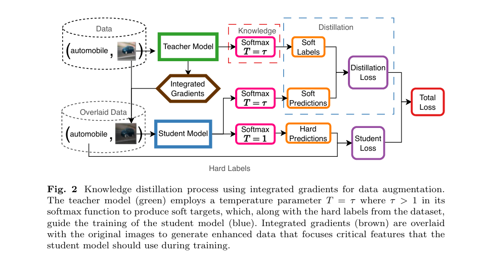
- A 4.1x compressed MobileNetV2 student trained with integrated gradient augmentation reaches 92.5% accuracy on CIFAR-10, beating both the standard student baseline (91.43%) and knowledge distillation alone (92.29%).
- The approach reduces inference latency from 140 ms to 13 ms, a 10.8x speedup, without any hardware-specific tricks.
- Integrated gradient maps are precomputed once before student training starts, so the runtime overhead is minimal.
- The optimal IG overlay probability is surprisingly low at p = 0.1. Anything above 0.25 hurts generalisation.
- Ablation results confirm that KD and IG augmentation contribute different and complementary signals, not redundant ones.
- The method works at the pixel level, giving the student model explicit visual hints rather than abstract probability distributions.
The Problem That Has Not Gone Away
Anyone who has tried to ship a decent image classifier on a microcontroller or a low-end phone knows the core tension. The models that perform well are enormous. The devices that need to run them are not. Quantisation and pruning chip away at parameters, but aggressive compression tends to degrade accuracy in nonlinear ways. Knowledge distillation, the technique where a compact student model learns from a larger teacher model, has become the standard middle ground, and it works well enough that most published benchmarks on CIFAR-10 report accuracy drops of well under one percentage point at moderate compression ratios.
But there is a gap in what knowledge distillation actually transfers. When the teacher passes soft probability distributions to the student, it is communicating which classes are similar, not which pixels or regions drove that conclusion. A soft label that reads 40% automobile, 35% truck, and 25% everything else tells the student something real about the decision boundary, but it says nothing about whether the model was looking at the wheels, the grille, or the silhouette. That is useful information, and standard KD throws it away.
The paper from Hernandez, Chang, and Nordling at arXiv:2503.13008v1 asks a reasonable question: what if you did not throw it away? What if you used the teacher’s own explainability output as a data augmentation signal, literally overlaying the attention map onto the training image before the student ever sees it?
Where Integrated Gradients Fit In
Integrated gradients (IG), introduced by Sundararajan, Taly, and Yan in 2017, is one of the more principled attribution methods in the explainability toolkit. The core idea is to accumulate gradient information along a straight path from a baseline input (typically a black image) to the actual input, measuring how much each pixel’s shift away from zero contributed to the final prediction. The result is a heatmap that satisfies two formal properties: sensitivity, meaning a pixel that changes the output is always attributed a nonzero value, and implementation invariance, meaning two functionally identical networks produce identical attributions regardless of their internal structure.
That rigor matters in a compression context because you need the attribution signal to be trustworthy. If the heatmap is unstable or depends on implementation quirks, overlaying it on training images introduces noise rather than signal. IG’s axiomatic guarantees give you some confidence that the bright regions in the map actually reflect the teacher’s decision process.
The formulation from the paper expresses this as a path integral over the prediction function F of the teacher model:
Here x is the input image, x’ is the baseline (black image), and the integral accumulates how the gradient of the prediction with respect to pixel i changes as you interpolate from baseline to input. In practice this integral is approximated with a finite number of steps, typically 50 to 300, which is why computing it for the entire training set is expensive enough to worry about.
Why This Differs From Attention Transfer
Attention transfer, used by Zhao et al. (2020) to reach 94.42% at 3.19x compression, guides the student by matching intermediate feature maps from the teacher. IG augmentation works earlier in the pipeline. Instead of adding a loss term that penalizes mismatched activations, it modifies the input data itself, letting the student’s own supervised training signal absorb the feature hint without any architectural coupling between teacher and student.
The Overlay Strategy: Simple and Specific
The way the team deploys IG is worth unpacking in detail, because the design choices are not obvious.
First, the maps are precomputed. Before student training begins, the team runs every training image through the teacher and computes its IG map. This converts what would be a per-batch attribution computation, at roughly 50 to 300 forward passes per image per step, into a one-time preprocessing cost that scales with dataset size, not training duration. On CIFAR-10 with 50,000 training images that is manageable. On ImageNet it would require more careful planning, but the principle holds.
Second, the map intensity is randomized with a log-uniform scale factor drawn from an exponential distribution between 1 and 2. The map is then normalized to the range zero to one. This prevents the overlay from always emphasizing regions at fixed contrast, which could encourage the student to latch onto a specific visual artifact rather than learning to recognize the underlying feature.
Third, the overlay itself is stochastic. With probability p, the final training image blends the original and the normalized IG map at equal weight:
The equal blend weight is a design choice worth scrutinizing. A heavier weight on the IG map would more aggressively highlight the discriminative region but would also distort the raw photometric signal the student relies on for other learned features. The authors do not report sensitivity to this blend ratio, which is a gap future work could fill.
The student model never sees a direct gradient from the teacher’s explainability system. It just sees images where important regions look slightly different, and it learns accordingly.
Paraphrase of the central mechanism from arXiv:2503.13008v1Knowledge Distillation as the Backbone
The IG overlay does not replace knowledge distillation, it augments it. The distillation loss keeps its standard form: a weighted sum of cross-entropy against hard labels and Kullback-Leibler divergence against the teacher’s softened output distribution.
$$\mathcal{L}_H = -\sum_i y_i \log f_s(x)_i$$
$$\mathcal{L}_{\text{KL}} = \sum_i f_t(x;T)_i \log \frac{f_t(x;T)_i}{f_s(x;T)_i}$$
The temperature parameter T softens the teacher’s probability distribution before the KL divergence is computed. A higher T spreads probability mass more evenly across classes, amplifying the inter-class similarity signal. A lower T preserves the hard, peaked distribution the teacher produces at inference time.
Through a grid search over 5 to 9 values of T, the distillation weight alpha, and the overlay probability p, the team found that T = 2.5 and alpha = 0.01 worked best. The low alpha is notable. It means hard labels still dominate the training signal, and the KL divergence term contributes a small corrective nudge. That makes sense on CIFAR-10, where the training labels are clean and reliable. On a noisier dataset the optimal alpha might shift upward.
Optimal Hyperparameter Summary
Temperature T = 2.5 balances class relationship preservation against categorical sharpness. Distillation weight alpha = 0.01 keeps hard labels dominant. IG overlay probability p = 0.1 provided the best generalization. Probabilities of 0.25 and 0.5 degraded accuracy, suggesting the student benefits from seeing clean, unadulterated images most of the time.
What the Numbers Actually Say
The teacher here is MobileNetV2 at 2.2 million parameters, trained to 93.91% on the CIFAR-10 test set. The student is a reduced version with 543,498 parameters, achieved by trimming both depth and width while preserving the early feature extraction layers. The 4.1x parameter ratio is more moderate than the most aggressive results in the literature, where Bhardwaj et al. (2019) reached 19.35x compression with a custom NoNN architecture, but it targets a different point on the tradeoff curve.
| Method | Accuracy (%) | Gain vs baseline |
|---|---|---|
| Teacher (MobileNetV2) | 93.91 | Reference |
| Baseline student (no distillation) | 91.43 | 0.00 |
| KD only | 92.29 | +0.86 |
| IG augmentation only | 92.01 | +0.58 |
| KD and IG combined | 92.45 | +1.02 |
The combined result preserves 98.4% of the teacher’s accuracy while using 24.3% of its parameters. The inference speedup is disproportionately large: latency drops from 140 ms to 13 ms, a 10.8x reduction despite only a 4.1x parameter reduction. The authors attribute this to reduced memory bandwidth requirements and better cache utilization in the smaller model, both of which scale nonlinearly with model size on modern GPU memory hierarchies.
| Model | Latency (ms) | Speedup |
|---|---|---|
| Teacher (MobileNetV2, 2.2M params) | 140 | 1.0x |
| Student (KD and IG, 543K params) | 13 | 10.8x |
The ablation results are arguably the most interesting piece of the paper. IG augmentation alone gives +0.58 percentage points. KD alone gives +0.86. The combination gives +1.02, which is less than the sum of the two individual gains. That sub-additive synergy suggests the two signals overlap partially, which is expected. Both ultimately try to help the student focus on what matters. But the fact that the combination still outperforms either alone confirms they contribute non-redundant information.
Reading the Broader Comparison
The paper situates itself well in the literature. Figure 1 in the original paper plots every comparison study as a line from teacher accuracy to student accuracy, with the x-axis as compression factor. The mean compression factor across the compared studies is 9.57x and the mean accuracy is 91.51%. This paper’s result sits at a lower compression factor (4.1x) but with accuracy above the mean.
The fairest comparison is probably against Zhao et al. (2020), which achieved 94.42% at 3.19x compression using a feature-highlighting approach called collaborative teaching, and against Su et al. (2022), which reached 94.69% at 3.26x. Both of those target a similar compression range and both outperform this paper in absolute accuracy. What this paper trades for its 2.0 to 2.2 percentage point deficit is a fundamentally different mechanism. It does not require intermediate feature matching between teacher and student, which means the teacher and student architectures can differ more freely. You do not need to align the activation dimensions of corresponding layers.
The comparison against Bhardwaj et al. (2019) is less direct. Their 19.35x compression at 94.53% accuracy uses a custom NoNN (neural network-on-neural-network) architecture designed for IoT deployment. The compression method is incommensurable with a general KD framework. Still, it is a useful reminder that 4.1x is a conservative compression target, and the team’s framing around edge computing would be strengthened by testing at higher compression ratios.
If you have been following our coverage on model compression and knowledge distillation, the pattern here fits a broader shift. The field is moving away from treating the student’s output distribution as the only thing that matters and toward richer representations of what the teacher actually learned. Attention transfer, hint-based distillation, and now IG augmentation are all variants of the same instinct: the soft labels are not enough, tell the student more.
A Reproducible PyTorch Implementation
Below is a complete, runnable implementation of the KD and IG augmentation pipeline. All components are present, including the IG precomputation, the augmented dataset, the distillation loss, the training loop, and a smoke test on dummy data.
Honest Limitations
What This Paper Does Not Settle
Dataset scope. Every experiment runs on CIFAR-10, a dataset with 32×32 images and 10 balanced classes. How the IG overlay generalizes to ImageNet, with its 224×224 images and 1,000 classes, is entirely unknown. The spatial structure of IG maps at higher resolution may behave very differently.
Compression ratio coverage. The 4.1x compression factor sits well below the literature mean of 9.57x. Whether the IG advantage holds or degrades at deeper compression is not tested. It is plausible that at very high compression ratios, the student’s limited capacity cannot absorb the pixel-level hints efficiently.
Blend weight sensitivity. The equal 50/50 blend between the original image and the IG map is a fixed design choice that the paper does not ablate. A heavier IG weight might help in some domains and hurt in others.
Computational cost of IG precomputation. The paper claims this is a manageable one-time cost on CIFAR-10. On a 50,000-image dataset with 50 integration steps per image, that is 2.5 million teacher forward passes before training even begins. On larger datasets this could become the bottleneck, and alternatives like smoothgrad or gradient-times-input might be worth comparing on both cost and augmentation quality.
Single architecture pair. MobileNetV2 teacher to a custom compact student is the only pair tested. Whether the method works when the teacher and student architectures are more architecturally dissimilar, say a ResNet-50 teacher to a small CNN student, is an open question.
Why This Matters for Edge Deployment
The practical argument for this method is straightforward. Most edge deployment pipelines already run some form of knowledge distillation. The only new engineering requirement here is a preprocessing step that generates and stores IG maps before training starts. The training loop itself does not change. The loss function does not change. The student architecture does not need to expose intermediate layers for matching. That is a low adoption cost for a consistent +0.5 to +1.0 percentage point accuracy gain.
The interpretability angle is genuinely useful, not just a selling point. When you deploy a compressed model to a medical device or a safety-critical system, knowing that the compressed model attends to the same image regions as the full model is a meaningful assurance. Attention transfer methods provide a similar guarantee implicitly, through matched feature maps. IG augmentation makes it explicit at the input level, which is easier to visualize and audit.
The connection to explainable AI is also worth noting for teams working on explainability-constrained deployments. If a regulation or an internal policy requires that a model’s decisions be attributable to specific input features, a student trained with IG augmentation inherits a documented feature-alignment relationship with the teacher model, which is a stronger audit trail than a model trained purely with soft labels.
Frequently Asked Questions
Read the full paper and run the official code from National Cheng Kung University’s NordlingLab.
Read on arXiv View Code on GitHubClosing Thoughts
The paper from Hernandez, Chang, and Nordling is a clean piece of applied research. The central idea, using explainability output as training-time augmentation rather than as a post-hoc inspection tool, is genuinely novel. Most prior work treats attribution methods as something you run after training to understand a model. This paper asks whether you can run them before training to improve one.
The results are encouraging but carefully scoped. A 4.1x compression ratio with a 98.4% accuracy retention rate and a 10.8x latency reduction is a solid outcome, but it is not the most aggressive compression in the literature. The paper wisely avoids overclaiming. The comparison figure makes clear that higher compression ratios exist, at the cost of accuracy, and that this method occupies a specific point on that frontier rather than redefining it.
The deeper contribution is methodological. By demonstrating that IG and KD contribute complementary non-redundant signals in the ablation study, the paper establishes a principle: feature-level attribution guidance is not just useful for human understanding, it is useful for machine learning. That principle could extend to other compression techniques, other attribution methods, and other tasks beyond image classification.
For practitioners, the immediate takeaway is pragmatic. If your pipeline already uses knowledge distillation, adding IG augmentation costs one preprocessing run and a minor change to the dataset loader. The accuracy gain is consistent and the mechanism is sound. The caveats are real: test it on your specific dataset and architecture before treating the CIFAR-10 numbers as a guarantee.
For the research community, the next obvious step is scale. Does this work at ImageNet resolution? Does it hold at 10x or 20x compression? Does the benefit transfer to tasks beyond classification? Those are questions worth answering, and this paper gives a credible starting point from which to answer them.
Related Articles
This analysis is based on the published paper and an independent evaluation of its claims.