
Key Points
- Standard keypoint distillation for 6DoF pose estimation treats all teacher predictions equally, transferring noise from uncertain keypoints into the student model alongside genuinely useful knowledge.
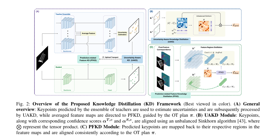
- UAKD (Uncertainty-Aware KD) uses a deep ensemble of teacher models to estimate per-keypoint epistemic uncertainty, then down-weights high-uncertainty keypoints in the optimal transport alignment between teacher and student.
- PFKD (Prediction-related Feature KD) reuses the same optimal transport plan to align teacher and student feature map regions, ensuring the prediction-level and feature-level distillation are consistent rather than independent.
- On LINEMOD with the lightest student (DarkNet-Tiny-H, 95.5% fewer parameters than the teacher), the combined method reaches an ADD-0.1d of 89.0, compared to 84.8 for the best prior method.
- On the SPEED+ spacecraft dataset, UAKD+PFKD closes the gap to the full teacher model in the synthetic domain and cuts the pose error by 0.120 in the lightbox domain versus the student baseline.
- An ensemble of just 4 to 6 teacher models is sufficient to approximate the true epistemic uncertainty, keeping inference overhead manageable during uncertainty estimation.
The Problem Everyone Was Ignoring
Think about what a keypoint detector actually does. It takes an image, runs it through a large backbone, and returns a set of 2D coordinates corresponding to corners or landmark points on a 3D object. Those coordinates feed into a PnP solver that recovers the full 6DoF pose. The quality of the final pose estimate is entirely hostage to the quality of those keypoints.
Now think about what knowledge distillation does in this context. The teacher model makes its keypoint predictions, and the student model is trained to match them through some alignment loss. The alignment in the best prior method, ADLP from Guo et al. (CVPR 2023), is formulated as an optimal transport problem, which is a principled way to match two sets of predictions that may not have the same cardinality. That is a real contribution.
But here is what both ADLP and the method before it from Guan et al. quietly assume: that every teacher prediction is worth imitating. In a heavily cluttered scene, or when the object is partially occluded, or at an awkward viewing angle, the teacher may predict keypoints it is genuinely unsure about. The keypoint might be projected onto a textureless surface. The teacher ensemble, if you run several of them, produces wildly spread predictions for that keypoint because no single model agrees on where it should be. Feeding that uncertain prediction into the distillation loss as confidently as a well-localized keypoint is, at best, wasteful. At worst, it actively misleads the student.
The University of Luxembourg team, working under the ELITE project funded by the Luxembourg National Research Fund (FNR) and in collaboration with Infinite Orbits, makes the observation that this is a fixable problem. Uncertainty is not just a nuisance to be ignored. It is information. And if you have it, you should use it.
When a teacher model is uncertain about a keypoint location, averaging that uncertainty into the distillation loss corrupts the student’s understanding of the task. The student learns not just where keypoints probably are, but also the teacher’s confusion about where they might be. UAKD treats uncertainty as a first-class signal and adjusts the distillation weight accordingly.
Getting Uncertainty Without a Bayesian Network
The first question anyone asks when uncertainty comes up is how you get it without rebuilding your network. Bayesian neural networks with learned weight distributions are expensive and change the architecture. Monte Carlo dropout approximates something, but its connection to true epistemic uncertainty is debated. The paper takes the practical route: deep ensembles.
An ensemble of four to six teacher models, each trained from a different random initialisation, is run at inference time on each input image. Each model produces its own set of predicted keypoint locations. For each keypoint, the spread of predictions across the ensemble tells you how much the teacher family disagrees about that keypoint’s location. That disagreement is epistemic uncertainty, meaning it comes from model parameter uncertainty rather than from irreducible noise in the data (aleatoric uncertainty). The distinction matters because epistemic uncertainty is something you can, in principle, reduce by training better, which means it reflects a genuine gap in the teacher’s knowledge about a particular region of the input space.
Per-keypoint variance is computed as the sum of the x and y coordinate variances across the ensemble. That raw variance is then passed through a tanh function to squeeze it into the range from 0 to 1, giving a scalar uncertainty score for each keypoint. High score means the ensemble disagrees. Low score means the ensemble converges.
The paper confirms that 4 to 6 models are sufficient to get a stable estimate of this epistemic uncertainty. This is an important practical result. Running six teacher models at training time adds overhead, but it does not require changing the network architecture, and the ensemble is only needed during distillation, not at deployment.
UAKD: Weighting the Optimal Transport Plan
With per-keypoint uncertainty scores in hand, the prediction-level distillation becomes an unbalanced optimal transport problem where the teacher’s keypoints are weighted by their confidence rather than treated uniformly. The confidence weight for each teacher keypoint is defined as one minus its uncertainty score, so a certain keypoint gets full weight and an uncertain one gets reduced weight in the alignment.
For models like WDRNet that also provide keypoint existence probabilities (a separate signal about whether a keypoint is likely to be visible at all), those probabilities can be blended with the uncertainty weights using a scalar factor lambda. The paper finds that an equal 50/50 blend (lambda equals 0.5) works best on LINEMOD, which suggests the two signals are complementary rather than redundant.
The unbalanced Sinkhorn algorithm then finds the optimal transport plan that minimises total alignment cost between the weighted teacher and student distributions. Because teacher keypoints with high uncertainty carry less weight, the optimal plan naturally focuses the distillation on the regions where the teacher is reliable. Uncertain keypoints still participate, but they pull less hard on the student’s learning trajectory.
This is mechanically clean. You do not need to threshold and discard uncertain keypoints, which would require choosing a cutoff and could discard useful signal. You just reduce their influence continuously, in proportion to how uncertain they are.
PFKD: Following the Keypoints Into the Feature Maps
The feature-level piece of the framework addresses a problem that predates this paper: feature-level and prediction-level distillation are almost always designed independently, with no coupling between them. You might align intermediate feature maps using some attention-based method, and separately align the output keypoint predictions using OT, and the two gradients are just summed together. There is nothing ensuring they point in the same direction.
PFKD (Prediction-related Feature KD) takes a different approach. Instead of selecting feature regions through a separate attention mechanism or heuristic, it traces each predicted keypoint back to its spatial receptive field in the feature map. Because the keypoint prediction head is a sequence of convolutions that preserve spatial structure, each output keypoint location corresponds to a well-defined region in the backbone feature map. The size of that region is determined by the kernel sizes and strides in the prediction head, which are fixed architectural constants.
Once teacher and student feature regions are identified for each keypoint, the PFKD loss aligns corresponding regions using the same optimal transport plan computed in UAKD. This is the key coupling. The OT plan already encodes which teacher keypoints match which student keypoints, weighted by uncertainty. Applying that same plan to the feature regions means that uncertain teacher keypoints, which are downweighted in the prediction-level OT, are also downweighted at the feature level. The two losses cannot pull in contradictory directions.
By reusing the OT plan from the prediction-level in the feature-level distillation, the framework avoids the inconsistency that plagues methods where prediction-level and feature-level objectives are designed in isolation. Paraphrase of the core architectural decision from Ousalah et al., 2025
When the teacher and student use different backbone channel counts, a 1×1 convolution adjusts the teacher’s feature channels to match, and average pooling adjusts the spatial dimensions. This is standard and adds minimal parameters.
Results on LINEMOD: Numbers That Tell a Story
You can read the full paper at arXiv:2503.13053, but the headline numbers deserve careful unpacking. The teacher model is WDRNet with a DarkNet-53 backbone, 52.1 million parameters and 36.51 billion FLOPs. The lightest student is WDRNet with DarkNet-Tiny-H, just 2.3 million parameters and 4.75 billion FLOPs. That is a 95.5% parameter reduction and an 87% FLOPs reduction. The question is how much accuracy survives.
| Method | Student Backbone | Params [M] | ADD-0.1d AVG | vs Teacher (92.9) |
|---|---|---|---|---|
| Student (no KD) | DarkNet-Tiny-H | 2.3 | 81.9 | ‑11.0 |
| ADLP + FKD | DarkNet-Tiny-H | 2.3 | 84.8 | ‑8.1 |
| UAKD only | DarkNet-Tiny-H | 2.3 | 88.1 | ‑4.8 |
| PFKD only | DarkNet-Tiny-H | 2.3 | 88.2 | ‑4.7 |
| UAKD + PFKD | DarkNet-Tiny-H | 2.3 | 89.0 | ‑3.9 |
| ADLP + FKD | DarkNet-Tiny | 8.5 | 90.4 | ‑2.5 |
| UAKD + PFKD | DarkNet-Tiny | 8.5 | 92.3 | ‑0.6 |
The improvement from 84.8 to 89.0 on the smallest student is not marginal. It is 4.2 points on a benchmark where a single point improvement over prior work is worth publishing. What is perhaps more striking is the DarkNet-Tiny result: UAKD+PFKD reaches 92.3 ADD-0.1d, which is within 0.6 points of the teacher’s 92.9 while using 83.7% fewer parameters. The student even surpasses the teacher on individual classes including Benchvise, Can, Driller, and Eggbox.
The ablation is honest about the contribution of each component. UAKD alone accounts for most of the gain. PFKD adds a smaller but consistent improvement on top. The combination is more than either alone, which is the expected result when two complementary mechanisms are combined. Neither component is doing the other’s job. For more context on how prediction-level and feature-level distillation interact, see [PLACEHOLDER — link to your knowledge distillation pillar or survey article].
SPNv2 and the Spacecraft Domain
The SPEED+ results are more interesting than LINEMOD in one respect: domain shift. The training data is synthetic and the evaluation domains (lightbox and sunlamp) use physical hardware to simulate orbital lighting conditions. The teacher SPNv2 model uses an EfficientDet-D6 backbone at 57.8 million parameters. The student uses EfficientDet-D0 at 3.8 million parameters, a 93.4% reduction, with FLOPs going from 288.27 billion down to 12.1 billion. That is a significant compression for a safety-critical application.
In the synthetic domain, UAKD+PFKD reaches a pose error of 0.024, matching the teacher exactly. In the lightbox domain, the student method reaches 0.248, compared to 0.202 for the teacher. That gap exists because a smaller model is less robust to lighting distribution shift, not because of a flaw in the distillation method. What matters is the comparison to the student without distillation (0.368) and to the ADLP+FKD baseline (0.336). UAKD+PFKD at 0.248 is a substantial improvement over both.
The sunlamp domain is the hardest, simulating direct solar illumination which creates sharp shadows and strong specular highlights. Here, UAKD+PFKD reaches a pose error of 0.360, compared to 0.388 for ADLP+FKD and 0.401 for the unassisted student. The rotation error reduction is 2.340 degrees compared to ADLP+FKD, which is meaningful for applications like satellite docking where angular precision is the primary constraint. For a broader look at where efficient models fit in robotics and space applications, see [PLACEHOLDER — link to your robotics pillar article].
What the Ablation on Lambda Actually Reveals
Figure 3 in the paper plots ADD-0.1d against different values of lambda, the weight that balances uncertainty scores against keypoint existence probabilities in WDRNet. For both DarkNet-Tiny-H and DarkNet-Tiny, performance peaks at lambda equals 0.5 and drops at the extremes.
The existence probability (from WDRNet’s built-in probabilistic sampling) tells you whether the keypoint is expected to be visible. The uncertainty score tells you whether the teacher is confident about the location when it does predict a keypoint. These two signals are different enough that neither alone captures everything, but similar enough that a 50/50 blend hits the sweet spot. The fact that lambda equals 1.0 (pure uncertainty, ignoring existence) is worse than the blend suggests the existence probability carries genuinely complementary information.
For SPNv2, which does not provide existence probabilities in the same form, the framework falls back to using only the uncertainty weights. This is handled cleanly in the formulation and does not require architectural changes.
Running 4 to 6 teacher models at training time adds real compute cost. The ablation confirms that going from 0 ensemble members (plain single-teacher distillation) to 4 or 6 gains about 0.2 to 0.5 ADD-0.1d from the ensemble effect alone, before uncertainty weighting is applied. The paper argues, correctly, that most of the performance gain is from the uncertainty-aware weighting rather than the ensemble averaging. This matters because if you already have an ensemble from other experiments, the uncertainty estimation is almost free. If you have to train the ensemble from scratch, budget for that compute upfront.
Where the Method Has Limits
The LINEMOD dataset uses 13 object classes, which is not a large evaluation set by modern standards. The objects span a reasonable range of shapes, from symmetric objects like Eggbox and Glue (which use the ADD-S metric instead of ADD to account for symmetry) to irregular objects like Driller and Phone. But LINEMOD images are relatively clean and the backgrounds are controlled compared to real industrial or outdoor settings.
The SPEED+ dataset is more challenging in the domain shift sense, but the object of interest (the Tango spacecraft mockup) is always the only object in the frame. There is no occlusion, no background clutter of similar objects, and no ambiguous viewpoints caused by nearby objects. Real debris tracking in orbit would present all of these challenges simultaneously.
The feature region computation in PFKD assumes that the keypoint prediction head is a straightforward sequence of spatial convolutions. Architectures that use deformable convolutions, non-local operations, or attention-based heads would break the clean receptive field calculation. Extending PFKD to those architectures requires either a different tracing mechanism or an approximation.
Finally, the ensemble requirement means the method is not immediately applicable to scenarios where only a single trained teacher model is available. If the teacher was trained once and no alternative initialisations exist, the uncertainty estimation needs to be adapted, potentially using dropout-based approximations or other post-hoc uncertainty methods.
Why Consistent Two-Level Distillation Matters Beyond This Paper
The PFKD contribution touches on something that the broader KD community has underappreciated. When you combine prediction-level and feature-level distillation, the two losses are optimised simultaneously during training. If they were designed independently, they can specify contradictory goals: one loss wants the feature at position X to look like the teacher’s feature at position X, while the other loss wants the student’s keypoint prediction to match a different teacher keypoint than the one at position X. These contradictions create gradient conflicts and add noise to training.
The PFKD solution, which is to use the same OT plan for both levels, is simple but requires the two levels to be designed together rather than bolted together afterwards. This is a design principle worth borrowing for any multi-objective distillation problem where prediction outputs can be traced back to feature locations, which includes object detection, segmentation, and depth estimation. For related work on how optimal transport is used in other distillation settings, see [PLACEHOLDER — link to your knowledge distillation pillar or survey article].
PyTorch Implementation
The following is a complete, reproducible implementation of the UAKD loss, the PFKD feature region extraction and alignment, and the combined training objective. It includes a smoke test on random dummy data. Replace the minimal stub models with your actual teacher and student architectures.
Conclusion
The central contribution of this paper is conceptually simple but practically important: not all teacher predictions deserve equal trust, and a knowledge distillation framework that treats them equally is transferring noise alongside knowledge. The UAKD framework puts a measurement of that noise (the ensemble disagreement mapped to a per-keypoint uncertainty score) directly into the optimal transport alignment, so that the student spends its learning capacity on the parts of the teacher’s knowledge that are genuinely reliable.
The PFKD extension solves a problem that most combined distillation frameworks ignore. When you optimise prediction-level and feature-level losses jointly, you want those losses to tell a consistent story. PFKD achieves this by inheriting the OT plan from UAKD, which means the feature alignment reflects the same uncertainty-weighted correspondences as the prediction alignment. The student cannot receive contradictory signals about which teacher predictions and which feature regions to emulate.
The transfer of this design principle to other regression tasks is straightforward wherever keypoints or anchor locations can be traced back to feature map receptive fields. Object detection, human pose estimation, and monocular depth estimation all have this structure. The uncertainty estimation via deep ensembles works on any architecture without modification, and four to six models is a manageable requirement in any research or applied setting where a teacher ensemble can be trained.
What remains open is performance under heavy occlusion, on multi-object scenes, and in the presence of ambiguous symmetries beyond the two symmetric objects in LINEMOD. The spacecraft use case, where this method was partly motivated by the Infinite Orbits collaboration, involves real orbital conditions that SPEED+ only approximates. Validation on actual space imagery or higher-fidelity simulation remains future work.
The gap between the 2.3 million parameter DarkNet-Tiny-H student and the 52.1 million parameter teacher has been cut from 11.0 ADD-0.1d points (without any distillation) to 3.9 points. That remaining 3.9 points is partly irreducible capacity difference and partly something future methods might address. Getting it this low, while retaining the energy and memory advantages that make small models worth deploying in the first place, is exactly the point.
Frequently Asked Questions
What is 6DoF pose estimation and why does model size matter?
6DoF pose estimation means recovering the full position (3 translational degrees) and orientation (3 rotational degrees) of an object relative to a camera. It is used in robotics, augmented reality, and space navigation. Model size matters because real deployments often run on embedded hardware, onboard satellites, or AR headsets where memory and power budgets are strict. A 52 million parameter model that works on a workstation is not deployable on an autonomous satellite without compression.
How does the paper estimate teacher uncertainty without retraining the network?
It uses a deep ensemble: four to six teacher models trained from different random initialisations on the same data. At inference, all models predict keypoints for a given image. The variance in those predictions, computed per keypoint as the sum of x and y coordinate variances across the ensemble, measures how much the teacher family disagrees. This disagreement is then mapped to a score in the range from 0 to 1 using a tanh function, giving a per-keypoint uncertainty estimate without modifying the network architecture.
What is the role of optimal transport in this framework?
Optimal transport (OT) finds the most efficient way to move probability mass from one distribution to another, minimising total transportation cost. Here, the teacher and student may predict different numbers of keypoints, so OT provides a principled way to match them without requiring one-to-one correspondence. The paper extends this to an unbalanced formulation where each teacher keypoint is weighted by its confidence (one minus uncertainty), so that uncertain teacher predictions receive less influence on the transport plan.
How does PFKD differ from standard feature-level knowledge distillation?
Standard feature distillation typically aligns entire feature maps or regions selected by separate attention mechanisms, independently of the prediction-level alignment. PFKD instead selects feature regions by tracing each predicted keypoint back to its receptive field in the backbone feature map, and then aligns those regions using the same optimal transport plan computed for prediction-level distillation. This means the feature alignment is geometrically grounded in the keypoint predictions and inherits the same uncertainty weighting, avoiding contradictory signals between the two loss levels.
What do the LINEMOD and SPEED+ results actually demonstrate?
On LINEMOD, the combined UAKD and PFKD method achieves an ADD-0.1d of 89.0 with a 2.3 million parameter student, versus 84.8 for the best prior method with the same student. With the 8.5 million parameter student, the method reaches 92.3, which is within 0.6 points of the 52 million parameter teacher. On SPEED+, the method matches the teacher in the synthetic domain and significantly reduces the pose error in the lightbox and sunlamp domains compared to the student trained without distillation, demonstrating that the gains hold under domain shift.
Can this framework be applied to pose estimation architectures other than WDRNet and SPNv2?
Yes, with some adaptation. The UAKD uncertainty estimation and optimal transport alignment work with any architecture that predicts 2D keypoints. The PFKD feature tracing requires that the prediction head be a sequence of spatial convolutions with known kernel sizes and strides, which is true for most standard keypoint detectors. Architectures using deformable convolutions or attention-based heads would need a modified tracing approach to identify the relevant feature regions.
Read the full paper from the University of Luxembourg and Infinite Orbits, or access the SPEED+ spacecraft pose estimation dataset directly.
Related Articles
Ousalah, N. A., Kacem, A., Ghorbel, E., Koumandakis, E., and Aouada, D. (2025). Uncertainty-Aware Knowledge Distillation for Compact and Efficient 6DoF Pose Estimation. arXiv preprint arXiv:2503.13053v2. Work supported by the National Research Fund (FNR), Luxembourg, under project C21/IS/15965298/ELITE, and by Infinite Orbits.
This analysis is based on the published paper and an independent evaluation of its claims.
Thanks for sharing. I read many of your blog posts, cool, your blog is very good.
I don’t think the title of your article matches the content lol. Just kidding, mainly because I had some doubts after reading the article.
Your point of view caught my eye and was very interesting. Thanks. I have a question for you.