
Key points
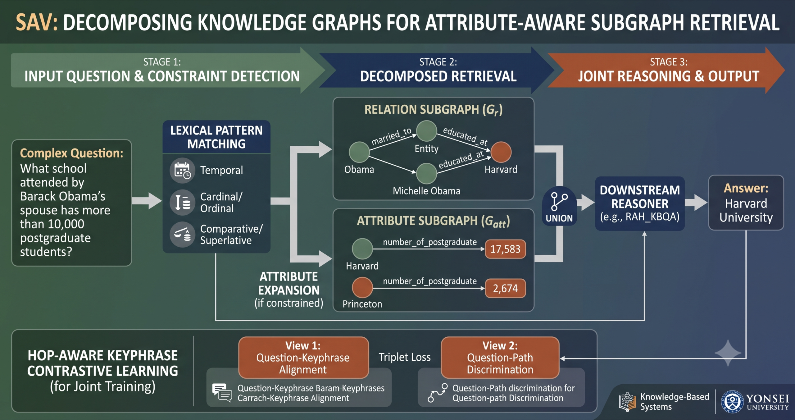
- SAV decomposes the KG into a relation graph of entity-to-entity triples and an attribute graph of entity-to-literal triples, then retrieves subgraphs from each separately for questions that require numerical or temporal constraints.
- Constrained question detection uses predefined lexical patterns covering temporal expressions, cardinal and ordinal numbers, and comparative and superlative cues. Attribute expansion is applied only when these patterns fire, keeping the overhead small.
- A Relation Path Tree built offline from weakly labeled training paths encodes how frequently each relation extension appears under a given prefix path. This structural prior is combined with learned semantic similarity during beam search to re-rank candidate relations at each hop.
- On CWQ, SAV* reaches H@1 of 66.2 and F1 of 65.7, outperforming Num (the closest attribute-aware baseline) by 8.6 points on H@1 and improving the constrained-question subset F1 from 48.3 to 57.3.
- Compared to LLM-based retrieval pipelines, SAV achieves higher F1 than both RoG and SubgraphRAG on CWQ and WebQSP while running substantially faster than RoG. Attribute expansion adds only 0.050 seconds per WebQSP question and 0.074 seconds per CWQ question to the relation-only baseline.
- The gap between retrieval improvement and QA improvement on constrained questions reveals that downstream reasoning is also a bottleneck. Improving path coverage rate from 54.1% to 69.8% does not translate proportionally to QA gains, and the paper explicitly calls for stronger attribute-aware reasoners as future work.
The gap between topological and semantic completeness in KG retrieval
A standard knowledge graph contains two qualitatively different types of edges. The first type connects entities to other entities through named relations, forming the relational backbone that most retrieval methods are built to traverse. The second type connects entities to literal values through attribute relations, recording concrete facts like a person’s birth date, an organization’s founding year, the number of students enrolled in a program, or the running time of a television episode.
For questions that ask about things or people, following entity-to-entity edges is usually sufficient. For questions that filter, rank, or aggregate based on properties, the literal values are the evidence that distinguishes the correct answer from plausible alternatives. Ask which school attended by Barack Obama’s spouse has more than 10,000 postgraduate students, and you can follow the “married to” and “educated at” edges to arrive at a set of school entities, but you cannot choose among them without the literal number attached to each school’s enrollment attribute.
The paper’s analysis of existing retrievers shows that this is not a minor edge case. On CWQ, a dataset built specifically for complex questions, 25.9% of test questions require some form of constraint involving dates, numbers, or ordinal selection. On WebQSP, which covers simpler questions, 11% of test questions are still constrained. Methods that retrieve only relation paths often produce subgraphs that are topologically connected to the right answer but missing the evidence needed to confirm it.
The problem statement as a formal decomposition
The standard KGQA problem asks the model to maximize the probability of the correct answer given the question and the full knowledge graph. Because the full graph is too large to reason over directly, an intermediate subgraph retrieval step is used to extract a compact relevant portion. The standard formulation treats the retrieved subgraph as a single undifferentiated object.
SAV refines this by splitting the retrieved evidence into two components. The relation subgraph captures the multi-hop path structure connecting topic entities to answer candidates. The attribute subgraph captures the literal-valued edges needed to satisfy temporal, ordinal, or aggregative constraints.
This decomposition is not just notational. It motivates separate retrieval mechanisms for each subgraph type and allows the attribute expansion to be applied conditionally, only when the question is detected as constrained, rather than adding overhead to every query.
Four modules that build the pipeline
Semantic matching path extraction
The first module generates weak supervision by finding which KG paths best match each training question. For each training question, candidate relation paths from topic entity to answer entity are enumerated and converted into natural-language sentences using the Path2Sentence verbalization procedure, which applies template-based conversion that produces readable noun phrases from symbolic relation sequences. Each candidate sentence and the original question are encoded by Sentence-BERT, and their cosine similarity determines which path is selected as the positive training signal and which lower-ranked candidates become negatives. For constrained questions, this process is extended to collect attribute paths connected to the answer entity, so the supervision explicitly reflects the need for literal-valued evidence.
Keyphrase selection through question-path matching
The second module identifies which spans of the question correspond to specific hops or attributes. It uses a masking approach where each token in the question is individually masked and the semantic shift of the question representation is measured. Tokens whose removal causes large representational changes are treated as salient, and adjacent salient tokens form candidate phrases.
These candidate phrases are then matched against the labeled path from the previous module. For a path with multiple hops, phrase combinations whose length matches the hop count are considered, and the combination scoring the highest alignment with the path elements is selected as the positive keyphrase set. This gives the model hop-aware supervision that links specific question phrases to specific KG expansion steps rather than treating the question as a monolithic query.
Two-view contrastive learning
The third module trains the RoBERTa-based retriever using two complementary triplet losses. The first view, question-keyphrase contrastive learning, teaches the model which phrases in the question are useful for retrieval. For each topic entity, the type-highlighted question, formed by appending the entity’s predicted KG type to the question, acts as the anchor, and the positive and negative keyphrase sets from the previous module form the training pairs.
The second view, question-path contrastive learning, teaches the model which KG edges should be selected at each hop. For each hop, the question is reformulated into a keyphrase-highlighted version that emphasizes the phrase assigned to that hop. This hop-specific query representation then anchors a triplet loss against the positive and negative path elements from the path extraction module.
The two losses are complementary in an important sense. The keyphrase loss reduces noise on the question side, helping the model decide what part of the question contains the relevant evidence. The path loss addresses discrimination on the KG side, helping the model rank the correct relation or attribute above competing candidates at each expansion step.
Subgraph retrieval with the Relation Path Tree
At inference time, the trained retriever expands relation paths hop by hop from topic entities using beam search with width 10, returning up to 10 paths per topic entity. At each hop, candidate outgoing relations are ranked by two signals. The first is the learned semantic similarity between the hop-specific keyphrase-highlighted question and the candidate relation. The second is a structural prior from the Relation Path Tree, an offline data structure built from the weakly labeled training paths that records how frequently each relation extension appears after a given partial path.
For questions detected as constrained, SAV then expands an attribute subgraph from entities in the relation subgraph, prioritizing entities based on their contextual relevance under the predicted type. Candidate attributes are matched against constraint-related keyphrases using the same learned semantic matching mechanism. The final subgraph passed to the downstream reasoner is the union of both components.
Experimental results, the full picture
Experiments run on CWQ (27,639 training questions, 3,531 test questions with 915 constrained) and WebQSP (2,848 training, 1,639 test with 180 constrained). All methods use Freebase. The retriever is fine-tuned from RoBERTa-base using RAdam at a learning rate of 5×10⁻⁵ for 10 epochs on a single NVIDIA Quadro RTX 6000 GPU. Sentence-BERT uses all-MiniLM-L6-v2 for path scoring.
Retrieval quality
| Method | CWQ Acr | CWQ #entity | WebQSP Acr | WebQSP #entity |
|---|---|---|---|---|
| PPR | 78.6 | 2,115 | 95.2 | 1,134 |
| SR | 83.7 | 362 | 88.3 | 98 |
| EPR | 80.4 | 23 | 82.1 | 13 |
| SAV | 90.9 | 330 | 93.2 | 92 |
SAV achieves the highest answer coverage rate on CWQ (90.9%) while keeping the subgraph substantially smaller than PPR (330 entities versus 2,115). EPR produces the smallest subgraphs but pays for it with lower coverage. The table illustrates a genuine tradeoff between coverage and compactness. SAV’s position, high coverage at intermediate size, is more practical for downstream reasoning than either extreme: a subgraph so large it contains too many irrelevant candidates, or so small it misses the correct answer outright.
Final QA performance
| Retrieval | CWQ H@1 | CWQ F1 | WebQSP H@1 | WebQSP F1 |
|---|---|---|---|---|
| PPR | 54.4 | 49.3 | 77.2 | 72.6 |
| EPR | 61.9 | 63.2 | 72.3 | 71.9 |
| SR | 52.6 | 50.0 | 70.3 | 68.4 |
| SAV (relation only) | 62.3 | 61.1 | 75.9 | 73.5 |
| Num* (attribute-aware baseline) | 57.6 | 53.3 | 78.1 | 73.9 |
| SAV* (with attributes) | 66.2 | 65.7 | 77.1 | 74.8 |
On CWQ, SAV* reaches the highest H@1 and F1 in the comparison. The contrast between SAV and Num is notable because both are attribute-aware. Num reaches 57.6 H@1 while SAV* reaches 66.2, a gap of 8.6 points, suggesting that the joint retrieval design with keyphrase alignment and the Relation Path Tree prior contributes substantially beyond simply adding attribute paths to the output. On WebQSP, Num* achieves the best H@1 (78.1) while SAV* achieves the best F1 (74.8). The paper’s explanation is that WebQSP questions are simpler and shorter, so relation-only retrieval already covers much of the necessary evidence and the marginal gain from attribute expansion appears more in precision-recall balance than in top-1 accuracy.
“Retrieval is therefore not the only bottleneck on the constrained subset, and stronger attribute-aware reasoners are still needed to fully exploit improved attribute subgraphs.” Jeon, Yeom, Park, Kim, Lee — Yonsei University, Knowledge-Based Systems 2026
Constrained questions specifically
| Retrieval | CWQ Acr | CWQ Pcr (constrained) | CWQ constr. H@1 | CWQ constr. F1 |
|---|---|---|---|---|
| PPR | 78.6 | — | 33.7 | 33.3 |
| EPR | 80.4 | — | 24.1 | 35.5 |
| SR | 83.7 | — | 27.8 | 30.1 |
| Num* | 78.6 | 54.1 | 46.2 | 48.3 |
| SAV* | 90.9 | 69.8 | 56.1 | 57.3 |
The path coverage rate comparison is where SAV’s attribute design is most clearly validated. On constrained questions, SAV achieves a Pcr of 69.8% against Num’s 54.1%, a 15.7 point improvement, showing that the jointly trained attribute-aware retrieval finds constraint-satisfying paths more reliably than Num’s attribute-only approach. The QA gains on constrained questions, 56.1 versus 46.2 on H@1 and 57.3 versus 48.3 on F1, are real and substantial. At the same time, the 15.7-point retrieval improvement produces roughly a 9-point QA improvement, not a proportional gain, which confirms the paper’s honest assessment that downstream reasoning is also a bottleneck.
LLM comparison
| Method | WebQSP H@1 | WebQSP F1 | CWQ H@1 | CWQ F1 | Retrieval time (s) |
|---|---|---|---|---|---|
| RoG | 85.7 | 70.8 | 62.6 | 56.2 | 0.743–0.956 |
| SubgraphRAG | 86.6* | 70.6 | 57.0* | 47.2 | 0.028–0.032 |
| SAV* | 77.1 | 74.8 | 66.2 | 65.7 | 0.432–0.842 |
SAV’s strongest claim against LLM-based methods is on F1. It achieves 74.8 F1 on WebQSP against RoG’s 70.8 and SubgraphRAG’s 70.6, and 65.7 F1 on CWQ against RoG’s 56.2 and SubgraphRAG’s 47.2. On H@1, RoG and SubgraphRAG are stronger on WebQSP (85.7 and 86.6 versus 77.1 for SAV), while SAV leads on CWQ H@1 (66.2 versus 62.6 for RoG and 57.0 for SubgraphRAG). SubgraphRAG is dramatically faster (under 0.035 seconds) because it uses a lightweight MLP with parallel triple scoring rather than sequential hop-by-hop expansion. SAV’s 0.432 second retrieval on WebQSP is slower than SubgraphRAG but substantially faster than RoG, and the attribute overhead is small: attribute expansion adds 0.050 seconds on WebQSP and 0.074 seconds on CWQ because it applies only to constrained questions over an already-retrieved set of entities.
What the ablation study reveals about the pipeline
The ablation study removes each of six components in turn and measures the resulting drop on CWQ and WebQSP. The largest single drops on CWQ come from removing weakly labeled path supervision (H@1 falls from 62.3 to 58.1, F1 from 61.1 to 56.7) and removing the Question-Keyphrase loss (the same sized drop: 58.1 and 56.7). Type prediction removal causes a moderate drop to 61.6 and 59.2. Removing keyphrase selection drops CWQ to 60.0 and 58.4. Removing the Relation Path Tree drops CWQ to 60.4 and 57.9. Removing the Question-Path loss drops CWQ to 58.8 and 57.3.
The fact that removing labeled path supervision and removing the Question-Keyphrase loss produce identical drops suggests they are tightly coupled. Without labeled paths, the keyphrase supervision itself has no good training signal to align to. On WebQSP, the drops are smaller for structural components like the Relation Path Tree (H@1 barely changes at 75.3 versus 75.9) while phrase-related components still affect F1, consistent with WebQSP being shorter and more direct in its phrasing. The two contrastive losses provide complementary coverage. The keyphrase loss reduces question-side ambiguity. The path loss sharpens KG-side candidate discrimination. Removing either hurts, but neither fully substitutes for the other.
The failure cases the paper documents honestly
The error analysis is one of the more candid parts of the paper and deserves attention for what it reveals about SAV’s structural limits. Two failure modes are identified and illustrated with real examples.
Incomplete joint attribute coverage
The first failure involves questions that require multiple attributes to be retrieved together to satisfy a temporal range condition. Consider a question asking which team David Beckham played for in 2011. Answering this correctly requires both a “from” attribute (start year of each contract period) and a “to” attribute (end year) to identify which team’s contract overlapped with 2011. SAV scores attribute candidates individually by semantic similarity, which means it can successfully retrieve the “from” attribute while failing to recognize that the “to” attribute is also required. The model includes only one side of the temporal range in the subgraph, causing the reasoner to return both LA Galaxy and Real Madrid instead of the correct answer alone. Fixing this requires a mechanism for jointly scoring related temporal attributes rather than evaluating each edge in isolation.
Implicit constraint interpretation
The second failure involves questions where the constraint is expressed implicitly in natural language without a direct surface mapping to a KG attribute. “Who was the first President of the United States during World War II?” requires the model to understand that “during” is a temporal filtering expression and to connect it to the start and end date attributes of presidential terms. SAV finds the explicit attribute “position_held.from” but does not connect “during World War II” to the overlapping temporal interval. The model returns George Washington, the first President by ordinal position, rather than Roosevelt, the first President whose term overlapped with the war. This is a semantic interpretation gap, not a retrieval gap, and addressing it likely requires either richer constraint-expression patterns or integration with a reasoning component that can interpret implicit temporal expressions.
Limitations
- Attribute expansion is applied only to questions detected as constrained via lexical patterns. Questions with implicit constraints, like “during World War II” without an explicit date, may not trigger the expansion even though they require literal-valued evidence.
- Candidate attribute edges are scored individually by semantic similarity. Questions requiring multiple related attributes to be retrieved jointly, such as both start and end dates of a temporal range, may retrieve only one side of the constraint.
- The evaluation is conducted on Freebase-based benchmarks (CWQ and WebQSP). The verbalization templates, constraint-expression patterns, and Relation Path Tree priors are built around Freebase’s schema and predicate naming conventions. Applying SAV to other knowledge graphs such as Wikidata or DBpedia would require adapting these components.
- The paper notes that string literals beyond numerical and temporal values (such as genre names or nationality strings) are not handled in the current attribute expansion module.
- The retrieval-reasoning gap on constrained questions suggests that improvements in retrieval quality do not fully translate to proportional QA gains. Stronger attribute-aware reasoners are needed downstream to exploit the improved attribute subgraphs fully.
A reference implementation
The code below implements the core novel components of SAV: the masking-based keyphrase saliency scoring, the two-view triplet contrastive loss, and the Relation Path Tree. The full paper is available here. For the smoke test, a minimal encoder stub replaces the actual RoBERTa and Sentence-BERT models to make the code runnable without downloading large pretrained weights.
# sav_reference.py
# Independent educational implementation of the SAV core components.
# Source paper: Jeon, Yeom, Park, Kim, Lee. SAV (Subgraph retrieval with Attribute Values).
# Knowledge-Based Systems 349 (2026) 116408. DOI 10.1016/j.knosys.2026.116408
# Not the authors' released code. Written from the method description.

import re
import torch
import torch.nn as nn
import torch.nn.functional as F
from collections import defaultdict
from typing import List, Dict, Tuple, Optional


# ──────────────────────────────────────────────────────────────────────────────
# Constrained question detection (Section 4.1)
# ──────────────────────────────────────────────────────────────────────────────

# Patterns from the paper: temporal expressions, cardinal/ordinal numbers,
# and comparative/superlative cues determine whether attribute expansion runs.
_TEMPORAL = re.compile(
    r"\b(after|before|during|in\s+\d{4}|since|until|between\s+\d{4}|"
    r"from\s+\d{4}|\d{4}\s+to\s+\d{4}|started|ended|founded)\b",
    re.IGNORECASE,
)
_CARDINAL_ORDINAL = re.compile(
    r"\b(first|second|third|last|most|least|more\s+than|fewer\s+than|"
    r"at\s+least|at\s+most|how\s+many|total|\d+,?\d+)\b",
    re.IGNORECASE,
)
_COMPARATIVE_SUPERLATIVE = re.compile(
    r"\b(highest|lowest|largest|smallest|oldest|newest|earliest|latest|"
    r"biggest|greater|less)\b",
    re.IGNORECASE,
)


def is_constrained_question(question: str) -> bool:
    """Detect whether a question requires attribute expansion.

    Uses the three lexical pattern families described in Section 4.1:
    temporal expressions, cardinal/ordinal numbers, and comparative/
    superlative cues. Returns True if any pattern fires.
    """
    return (
        bool(_TEMPORAL.search(question))
        or bool(_CARDINAL_ORDINAL.search(question))
        or bool(_COMPARATIVE_SUPERLATIVE.search(question))
    )


# ──────────────────────────────────────────────────────────────────────────────
# Masking-based keyphrase saliency scoring (Section 4.2, equation 4)
# ──────────────────────────────────────────────────────────────────────────────

class MaskingKeyphraseExtractor:
    """Estimates token saliency by measuring how much each token's removal
    changes the sentence embedding. High saliency tokens are grouped into
    candidate keyphrases. Requires a callable encoder that maps a string
    to a unit-normalized embedding tensor.
    """

    def __init__(self, encoder, mask_token="[MASK]", threshold=0.05):
        self.encoder = encoder
        self.mask_token = mask_token
        self.threshold = threshold

    def token_saliencies(self, question: str) -> List[Tuple[str, float]]:
        """Return (token, saliency_score) pairs for every token in the question."""
        tokens = question.split()
        v_q = self.encoder(question)

        results = []
        for i, tok in enumerate(tokens):
            masked = " ".join(
                (self.mask_token if j == i else t) for j, t in enumerate(tokens)
            )
            v_masked = self.encoder(masked)
            # Equation 4: sim(q, q_masked) = V_q^T * V_q_masked
            score = float((v_q * v_masked).sum())     # cosine sim if unit-normed
            saliency = 1.0 - score                   # lower sim = higher saliency
            results.append((tok, saliency))
        return results

    def extract_keyphrases(self, question: str) -> List[str]:
        """Group adjacent high-saliency tokens into candidate key phrases."""
        pairs = self.token_saliencies(question)
        phrases, current_phrase = [], []
        for tok, sal in pairs:
            if sal >= self.threshold:
                current_phrase.append(tok)
            else:
                if current_phrase:
                    phrases.append(" ".join(current_phrase))
                    current_phrase = []
        if current_phrase:
            phrases.append(" ".join(current_phrase))
        return phrases


# ──────────────────────────────────────────────────────────────────────────────
# Two-view triplet contrastive loss (Section 4.3, equations 6-8)
# ──────────────────────────────────────────────────────────────────────────────

class TwoViewContrastiveLoss(nn.Module):
    """Combines the Question-Keyphrase and Question-Path triplet losses.

    Both losses use the same triplet formulation:
        L = max(0, margin + sim(anchor, negative) - sim(anchor, positive))

    View 1 (keyphrase): anchor = type-highlighted question (tq_i)
                        positive = matched keyphrase set (KP_i)
                        negative = mismatched keyphrase set (KPbar_i)

    View 2 (path):      anchor = keyphrase-highlighted question (kq_n_i)
                        positive = labeled path element (p_n_i)
                        negative = competing path element (pbar_n_i)

    Both anchors, positives, and negatives are represented as unit-normalized
    d-dimensional embedding vectors from the encoder.
    """

    def __init__(self, margin=0.1, lam=1.0):
        super().__init__()
        self.margin = margin
        self.lam = lam    # λ balancing keyphrase and path views (equation 8)

    def triplet(self, anchor, positive, negative):
        """Margin-based triplet loss (shared by both views)."""
        sim_pos = (anchor * positive).sum(dim=-1)   # cosine similarity (unit vecs)
        sim_neg = (anchor * negative).sum(dim=-1)
        return F.relu(self.margin + sim_neg - sim_pos)

    def forward(
        self,
        tq: torch.Tensor,        # (B, d) type-highlighted question embeddings
        kp_pos: torch.Tensor,    # (B, d) positive keyphrase embeddings
        kp_neg: torch.Tensor,    # (B, d) negative keyphrase embeddings
        kq: torch.Tensor,        # (B, d) keyphrase-highlighted question embeddings
        path_pos: torch.Tensor,  # (B, d) positive path element embeddings
        path_neg: torch.Tensor,  # (B, d) negative path element embeddings
    ) -> Tuple[torch.Tensor, torch.Tensor, torch.Tensor]:
        l_kp = self.triplet(tq, kp_pos, kp_neg).mean()   # equation 6
        l_path = self.triplet(kq, path_pos, path_neg).mean()  # equation 7
        total = l_kp + self.lam * l_path                   # equation 8
        return total, l_kp, l_path


# ──────────────────────────────────────────────────────────────────────────────
# Relation Path Tree (Section 4.4)
# ──────────────────────────────────────────────────────────────────────────────

class RelationPathTree:
    """Offline structural prior built from weakly labeled training paths.

    Stores how frequently each relation extension appears after a given
    prefix path. During inference, these normalized branch frequencies
    are used to re-rank semantically scored candidates.

    Example: if the prefix path is ['educated_at'] and 'number_of_postgraduate'
    appears 80% of the time as the next attribute while 'date_founded' appears
    20% of the time, the structural prior will favor 'number_of_postgraduate'
    under this prefix even if semantic similarity scores are comparable.
    """

    def __init__(self):
        # Maps prefix_tuple -> {next_relation: count}
        self._tree: Dict[Tuple, Dict[str, int]] = defaultdict(lambda: defaultdict(int))

    def add_path(self, path: List[str]):
        """Register one labeled path from training data.
        Each prefix of the path is updated with the next relation count.
        """
        for i in range(len(path)):
            prefix = tuple(path[:i])
            next_rel = path[i]
            self._tree[prefix][next_rel] += 1

    def build_from_dataset(self, labeled_paths: List[List[str]]):
        """Build the tree from a list of training paths."""
        for path in labeled_paths:
            self.add_path(path)

    def get_prior(self, prefix: List[str], candidates: List[str]) -> Dict[str, float]:
        """Return normalized frequency priors for each candidate relation.

        Returns uniform 1/|candidates| if the prefix was never seen in training.
        """
        prefix_key = tuple(prefix)
        counts = self._tree.get(prefix_key, {})
        total = sum(counts.values())
        if total == 0:
            uniform = 1.0 / max(len(candidates), 1)
            return {c: uniform for c in candidates}
        return {c: counts.get(c, 0) / total for c in candidates}

    def combined_score(
        self,
        prefix: List[str],
        candidates: List[str],
        semantic_scores: List[float],
        alpha: float = 0.7,
    ) -> Dict[str, float]:
        """Blend semantic similarity with the structural prior.

        alpha controls how much weight goes to the semantic score
        versus the structural frequency prior. The paper uses these
        as additive re-ranking signals rather than a fixed blend.
        """
        priors = self.get_prior(prefix, candidates)
        return {
            c: alpha * sem + (1 - alpha) * priors[c]
            for c, sem in zip(candidates, semantic_scores)
        }


# ──────────────────────────────────────────────────────────────────────────────
# Simplified SAV retriever (concept demo)
# ──────────────────────────────────────────────────────────────────────────────

class SAVRetriever:
    """Lightweight SAV inference pipeline.

    In a real deployment, the encoder is a fine-tuned RoBERTa-base model.
    Here we accept any callable encoder for testing.
    """

    def __init__(self, encoder, relation_path_tree: RelationPathTree, beam_width=10):
        self.encoder = encoder
        self.tree = relation_path_tree
        self.beam_width = beam_width
        self.keyphrase_extractor = MaskingKeyphraseExtractor(encoder)

    def _score_candidates(
        self, query_emb: torch.Tensor, candidates: List[str], prefix: List[str]
    ) -> List[Tuple[str, float]]:
        """Score each candidate relation/attribute by combined semantic+structural score."""
        sem_scores = []
        for c in candidates:
            c_emb = self.encoder(c)
            sem_scores.append(float((query_emb * c_emb).sum()))
        combined = self.tree.combined_score(prefix, candidates, sem_scores)
        return sorted(combined.items(), key=lambda x: -x[1])

    def retrieve(
        self,
        question: str,
        topic_entities: List[str],
        relation_graph: Dict[str, List[str]],  # entity -> list of (relation, target)
        attribute_graph: Dict[str, List[str]], # entity -> list of (attribute, value)
        max_hops: int = 2,
    ) -> Tuple[List[Tuple], List[Tuple]]:
        """Return (relation_subgraph_triples, attribute_subgraph_triples).

        Relation subgraph: hop-by-hop beam expansion from topic entities.
        Attribute subgraph: expanded from relation-subgraph entities for
                            constrained questions only.
        """
        keyphrases = self.keyphrase_extractor.extract_keyphrases(question)
        q_emb = self.encoder(question)

        # Relation subgraph expansion (beam search)
        relation_triples = []
        relation_entities = set(topic_entities)
        beams = [(e, []) for e in topic_entities]  # (current_entity, path_so_far)

        for _ in range(max_hops):
            next_beams = []
            for entity, prefix in beams:
                neighbors = relation_graph.get(entity, [])
                if not neighbors:
                    continue
                relations = [r for r, _ in neighbors]
                scored = self._score_candidates(q_emb, relations, prefix)
                for rel, score in scored[:self.beam_width]:
                    targets = [t for r, t in neighbors if r == rel]
                    for target in targets:
                        relation_triples.append((entity, rel, target))
                        relation_entities.add(target)
                        next_beams.append((target, prefix + [rel]))
            beams = next_beams[:self.beam_width]

        # Attribute subgraph expansion (constrained questions only)
        attribute_triples = []
        if is_constrained_question(question):
            for entity in relation_entities:
                attrs = attribute_graph.get(entity, [])
                if not attrs:
                    continue
                attr_names = [a for a, _ in attrs]
                for kp in keyphrases:
                    kp_emb = self.encoder(kp)
                    scored_attrs = self._score_candidates(kp_emb, attr_names, [])
                    for attr, score in scored_attrs[:3]:
                        values = [v for a, v in attrs if a == attr]
                        for val in values:
                            attribute_triples.append((entity, attr, val))

        return relation_triples, attribute_triples


# ──────────────────────────────────────────────────────────────────────────────
# Smoke test
# ──────────────────────────────────────────────────────────────────────────────

def smoke_test():
    # Minimal encoder stub: random unit-normalized vectors for any string
    torch.manual_seed(42)
    embedding_cache = {}

    def stub_encoder(text: str) -> torch.Tensor:
        if text not in embedding_cache:
            vec = torch.randn(128)
            embedding_cache[text] = F.normalize(vec, dim=0)
        return embedding_cache[text]

    # --- Test constrained question detection ---
    constrained = [
        "Which school attended by Barack Obama's spouse has a total number of students over 10,000?",
        "What movie with a running time of less than 60 minutes features Taylor Lautner?",
        "Where did Eleanor Roosevelt attend school, with a founding date of 1919?",
    ]
    unconstrained = [
        "Who is Barack Obama married to?",
        "What country is Germany located in?",
    ]
    for q in constrained:
        assert is_constrained_question(q), f"Should be constrained: {q}"
    for q in unconstrained:
        assert not is_constrained_question(q), f"Should be unconstrained: {q}"
    print("Constrained question detection: passed")

    # --- Test two-view contrastive loss ---
    loss_fn = TwoViewContrastiveLoss(margin=0.1, lam=1.0)
    B, d = 4, 128
    tq = F.normalize(torch.randn(B, d), dim=-1)
    kp_pos = F.normalize(torch.randn(B, d), dim=-1)
    kp_neg = F.normalize(torch.randn(B, d), dim=-1)
    kq = F.normalize(torch.randn(B, d), dim=-1)
    path_pos = F.normalize(torch.randn(B, d), dim=-1)
    path_neg = F.normalize(torch.randn(B, d), dim=-1)
    total, l_kp, l_path = loss_fn(tq, kp_pos, kp_neg, kq, path_pos, path_neg)
    total.backward()
    print(f"Two-view contrastive loss: total={total.item():.4f}, L_kp={l_kp.item():.4f}, L_path={l_path.item():.4f}")

    # --- Test Relation Path Tree ---
    tree = RelationPathTree()
    training_paths = [
        ["educated_at", "number_of_postgraduate"],
        ["educated_at", "number_of_postgraduate"],
        ["educated_at", "date_founded"],
        ["married_to", "educated_at", "number_of_postgraduate"],
    ]
    tree.build_from_dataset(training_paths)
    prior = tree.get_prior(["educated_at"], ["number_of_postgraduate", "date_founded"])
    assert prior["number_of_postgraduate"] > prior["date_founded"], \
        "number_of_postgraduate should have higher prior under educated_at prefix"
    print(f"Relation Path Tree: priors = {prior}")

    # --- Test end-to-end retrieval on toy graph ---
    relation_graph = {
        "Barack Obama": [("married_to", "Michelle Obama")],
        "Michelle Obama": [
            ("educated_at", "Princeton University"),
            ("educated_at", "Harvard University"),
        ],
    }
    attribute_graph = {
        "Princeton University": [("number_of_postgraduate", "2674")],
        "Harvard University": [("number_of_postgraduate", "17583")],
    }
    retriever = SAVRetriever(stub_encoder, tree, beam_width=5)
    q = constrained[0]
    rel_triples, attr_triples = retriever.retrieve(
        q, ["Barack Obama"], relation_graph, attribute_graph, max_hops=2
    )
    print(f"Retrieved {len(rel_triples)} relation triples and {len(attr_triples)} attribute triples.")
    print(f"Sample relation triples: {rel_triples[:3]}")
    print(f"Sample attribute triples: {attr_triples[:3]}")
    print("Full smoke test passed.")


if __name__ == "__main__":
    smoke_test()
Conclusion
The central claim of SAV is that knowledge graph question answering retrievers are making a systematic error: they retrieve the right entities via relation paths but omit the literal-valued attributes those entities carry, which are exactly what constrained questions need to distinguish the correct answer. The paper formalizes this as a decomposition of the KG into a relation graph and an attribute graph, trains a retriever that learns to align question phrases with both types of evidence through hop-aware contrastive learning, and adds a conditional attribute expansion step that activates only when the question is detected as constrained.
The results on constrained questions are the strongest part of the evidence. The 15.7-point improvement in path coverage rate over Num shows that joint relation-attribute retrieval with keyphrase alignment is substantially more effective than adding attribute paths as an afterthought. The downstream QA gain of about 9 points on constrained CWQ questions demonstrates that this retrieval improvement is real and actionable, not just a measurement artifact. The honest acknowledgment that the retrieval gain does not fully transfer to QA gains, and that stronger attribute-aware reasoners are needed, is the kind of precise limitation identification that makes a paper useful for follow-on work.
The Relation Path Tree is an underappreciated component of the design. It is not a learned model and requires no training of its own, but it encodes exactly the kind of structural pattern knowledge that semantic similarity alone cannot capture: the frequency with which specific relation sequences appear in real question-answering paths. Combining this offline structural prior with the learned semantic similarity produces a retrieval signal that is robust to cases where a relation is semantically plausible for the question but rarely seen in the path context the question implies.
The two failure modes documented in the error analysis are precisely specified and productive for future work. Incomplete joint attribute coverage, where scoring attributes individually misses multi-attribute constraints like temporal ranges, points toward joint attribute scoring or constraint template extraction as a direction. Implicit constraint interpretation, where “during World War II” does not trigger the right attribute alignment, points toward richer constraint-expression patterns or integration with a reasoning component that can unpack implicit temporal conditions into explicit KG attribute queries.
For practitioners, the most actionable finding is the overhead number. Adding attribute expansion to a relation-only retrieval pipeline costs 50 milliseconds per WebQSP question and 74 milliseconds per CWQ question, because expansion applies only to constrained questions and only over entities already retrieved. That is a small price for a 15-point path coverage improvement on the constrained subset, and the detection mechanism is simple enough to tune or extend for other constraint types beyond the temporal, ordinal, and aggregative categories covered here.
Frequently asked questions
What is the difference between the relation subgraph and the attribute subgraph in SAV
The relation subgraph contains entity-to-entity triples: facts like “Obama married Michelle” or “Michelle attended Princeton.” These form the relational backbone connecting topic entities to answer candidates. The attribute subgraph contains entity-to-literal triples: facts like “Princeton has 2,674 postgraduate students” or “an organization was founded in 1919.” These provide the numerical or temporal values needed to filter or rank among candidates when the question imposes a constraint.
How does SAV decide whether to expand an attribute subgraph
It uses predefined lexical patterns over the question text. If the question contains temporal expressions (“after,” “before,” “during,” “in 1919”), cardinal or ordinal numbers (“first,” “more than 10,000”), or comparative and superlative cues (“most,” “oldest,” “largest”), the question is classified as constrained and attribute expansion is applied. If none of these patterns match, only the relation subgraph is retrieved.
What is the Relation Path Tree and why does it matter
The Relation Path Tree is an offline data structure built from weakly labeled training paths. It records, for each prefix of relation steps seen in training, how frequently each possible next-hop relation appeared. During inference this structural frequency prior is combined with the learned semantic similarity score to re-rank candidate relations at each expansion step. A candidate that is both semantically aligned with the question and frequently observed under the current path context receives a higher combined score than one that scores well on only one criterion.
How does SAV compare to LLM-based KGQA pipelines
SAV achieves higher F1 than both RoG and SubgraphRAG on CWQ and WebQSP while running faster than RoG. On H@1, RoG and SubgraphRAG outperform SAV on WebQSP. SubgraphRAG is substantially faster (under 35 milliseconds per question) than SAV because it uses a lightweight MLP with parallel triple scoring rather than sequential hop-by-hop expansion. The trade-off is that SAV’s constrained-question performance is stronger, while SubgraphRAG is better suited for high-throughput simpler questions.
What are SAV’s two main failure modes
The first is incomplete joint attribute coverage. When a question requires two related temporal attributes together, such as both the start and end year of a contract to determine whether it overlapped with a given year, SAV may retrieve only one of them because it scores each attribute edge independently. The second is implicit constraint interpretation. When a constraint is expressed indirectly in natural language, such as “during World War II” rather than explicit years, SAV may fail to connect the implicit expression to the explicit KG attributes needed to represent it.
Read the full method, case studies, and error analysis in the source paper.