
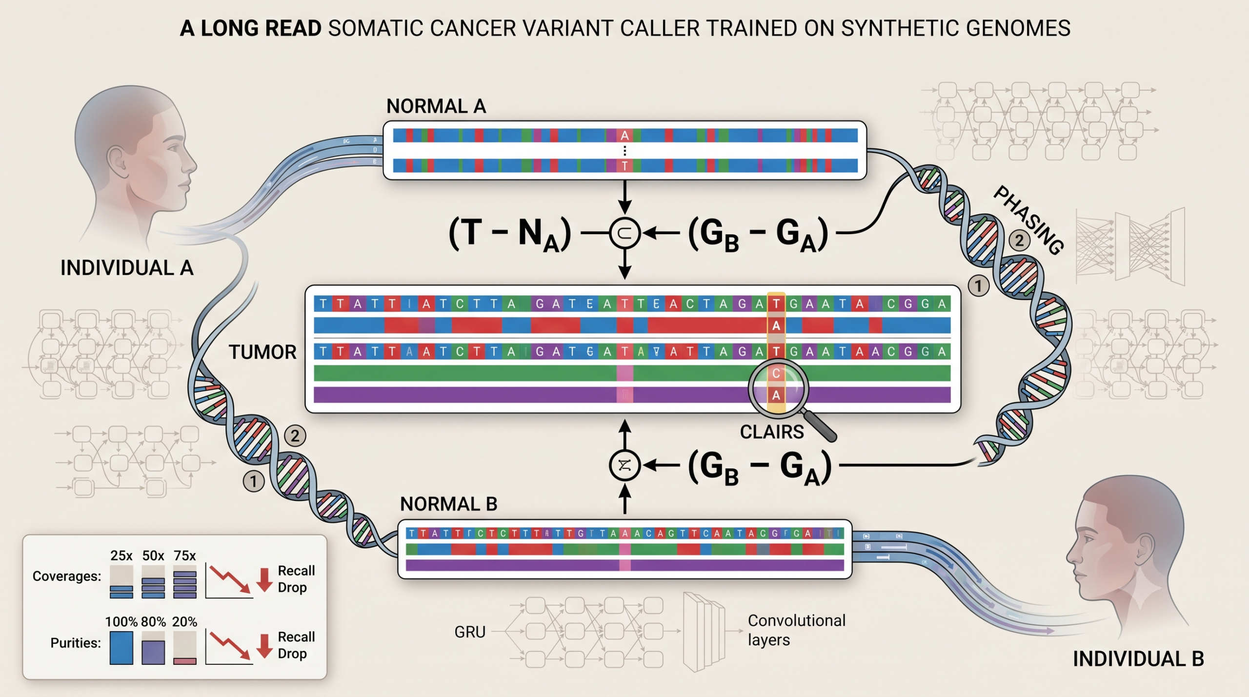
This article explains a published bioinformatics paper. ClairS is a research tool for detecting cancer mutations in sequencing data, it is not a diagnostic device and is not used on its own to make decisions about an individual patient’s care. Any clinical application of a variant caller like this would sit inside a larger, validated clinical pipeline with oversight from qualified laboratory professionals.
Key points
- ClairS is trained mostly on synthetic tumor and normal pairs built by combining two unrelated healthy genomes, since real cancer samples with known truth mutations are extremely scarce compared to the germline variant catalogs used to train other genomic AI tools.
- On the SEQC2 reference tumor pair HCC1395 and HCC1395BL at 50 times tumor and 25 times normal coverage, ClairS reached F1 scores of 89.83 percent for single nucleotide variants and 73.38 percent for indels, rising to 96.19 percent and 79.67 percent once real cancer cell lines were added to training.
- Long read phasing, the ability to tell which parental chromosome a read came from, is the single biggest lever in the whole pipeline. Turning it off drops the F1 score by 2.48 points, and removing the pileup network entirely drops it by nearly 8 points.
- Sensitivity collapses hard at low tumor purity. Recall fell from 86.86 percent at 100 percent tumor purity down to 22.43 percent at 20 percent purity in the balanced precision mode, a number worth knowing before assuming this tool works equally well on any biopsy.
- ClairS was trained and tested entirely on cancer cell lines, which have cleaner DNA than real patient tumor tissue, and the authors are explicit that performance on degraded, paraffin embedded clinical specimens remains untested.
The data problem nobody talks about
Cancer genome sequencing has a specific kind of AI training problem that most medical imaging models do not face. Germline variant callers, the tools that find inherited genetic differences, get to train on GIAB, the Genome In A Bottle reference collection, which supplies roughly 25 million confirmed truth variants across seven well studied samples. Somatic variant callers, the tools built to find mutations that arose only inside a tumor and are absent from that same patient’s healthy tissue, have almost nothing comparable. The single most trusted reference for this task, a breast cancer cell line called HCC1395 paired with its matched normal cell line HCC1395BL, published by the Sequencing Quality Control Phase 2 consortium, contains only 39,560 confirmed single nucleotide variants and 1,922 indels. That is orders of magnitude short of what a deep neural network typically needs.
Short read sequencing had a partial workaround called Bamsurgeon, which spikes artificial mutations directly into real sequencing alignments. It does not translate to long read platforms like Oxford Nanopore Technologies, for two concrete reasons the paper lays out. Nanopore reads are basecalled from a sliding signal window covering five or six bases at once, and once a read has been converted from raw electrical signal into DNA bases, there is no way to authentically convert it back to insert a spike in mutation, the signal simply cannot be reconstructed. Second, and more specific to long reads, Bamsurgeon does not respect the fact that a genuine somatic mutation almost always sits on only one of the two parental chromosome copies, while a sequencing artifact has no such constraint. Long reads are long enough to actually detect which chromosome copy a mutation sits on, called phasing or haplotyping, and any synthetic data generator that ignores this loses the one advantage long reads offer over short reads for this exact task.
The trick, two strangers’ genomes pretending to be one tumor
ClairS solves the data scarcity problem with an observation that sounds almost too simple once stated. A germline variant that is unique to one person looks, from a purely genetic standpoint, exactly like a somatic mutation when that person’s genome is compared against someone else entirely. Take a variant found only in individual A’s genome and never in individual B’s genome, treat A’s sequencing reads as tumor and B’s as the matched normal, and that inherited variant is now, computationally, indistinguishable from a real somatic mutation that arose only in the tumor.
The team used two GIAB reference samples, HG002 sequenced by Nanopore’s own EPI2ME Labs team at 76.29 times coverage, and HG001 sequenced at the University of Hong Kong at 48.44 times coverage. Both directions were used, HG001 as tumor against HG002 as normal, and the reverse. Reads from each sample were split into small four times coverage chunks, then recombined in different numbers and ratios to simulate practically any sequencing coverage, tumor purity, or level of normal cell contamination the team wanted, all from just two source genomes.
Comparing the resulting synthetic tumor and normal call sets against each sample’s known true germline variants sorts every candidate into one of four buckets.
Using T for the synthetic tumor call set, NA for the synthetic normal call set built from sample A, and GA, GB for the known true germline variants of samples A and B
$$ \text{somatic} = (T – N_A) \cap (G_B – G_A) $$ $$ \text{germline} = T \cap N_A \cap G_A \cap G_B $$ $$ \text{artifact} = T – N_A – G_A – G_B $$A candidate lands in the somatic bucket only if it shows up in the synthetic tumor, is absent from the matched synthetic normal, and is a real germline variant that belongs to sample B but not sample A. That last condition is what makes the trick work, it forces the synthetic somatic call to come from an actual biological variant, not sequencing noise. The germline bucket catches variants both samples genuinely share, and the artifact bucket catches everything left over, meaning it appeared in the tumor for no traceable biological reason and is therefore treated as training data for sequencing noise the network needs to learn to reject.
This process generated 12,489,342 training examples after several quality filters, a number the paper reaches specifically because a germline variant based approach can theoretically produce an unlimited supply, unlike waiting for more real tumor samples to become available. Subsampling the resulting variant allele fraction distribution toward a beta distribution shaped by parameters matching prior work from the SEQC2 consortium added a further 1.8 percent to the F1 score, since raw synthetic data tends to cluster around a few obvious allele fractions rather than the smooth continuous spectrum real tumors actually show.
Why this matters
DeepSomatic, a competing somatic caller released in late 2024, took the opposite approach, training directly on a diverse set of real cancer cell lines across multiple sequencing technologies. That approach genuinely captures cancer specific mutational signatures the synthetic method cannot, things like the particular length distribution of insertions and deletions in real tumors. ClairS’s answer is not to pick one strategy over the other, the final released model actually combines both, starting from the synthetic model and then fine tuning on four real tumor and normal cell line pairs, which the paper’s own numbers show is better than either approach alone.
Three steps from raw reads to a called mutation
Step one, phase the germline variants first
Before ClairS looks for anything resembling a mutation, it runs Clair3, the team’s own earlier germline variant caller, on both the tumor and normal samples to find high confidence heterozygous germline variants, using a stricter cutoff than Clair3’s own default, requiring variant allele fraction of at least 0.2 and coverage of at least 10. Only the heterozygous variants both samples share get used for phasing. The tool LongPhase then uses those shared variants to sort tumor reads into haplotype 1, haplotype 2, or unknown, a roughly fifteen times faster alternative to the older WhatsHap tool that the team found delivers comparable phase set lengths on human samples. Deliberately, ClairS never phases the normal sample’s alignments, since the team’s own experiment showed doing so doubled processing time without any accuracy gain.
Step two, two neural networks that are trusted equally
Every candidate position that clears an initial filter gets sent through two separate neural networks at once, a design choice that breaks from how ClairS’s own germline predecessor Clair3 operates.
A position is selected as a variant candidate for the networks to examine if it satisfies either of two conditions, where D denotes read depth, T is tumor, N is normal, and m is the alternative base being considered
$$ D^T_m \geq 3 \text{ and } \frac{D^T_m}{\sum_i D^T_i} \geq \alpha \text{ and } \frac{D^N_m}{\sum_i D^N_i} < \alpha $$ $$ \text{or } \quad D^T_m \geq 3 \text{ and } \frac{D^T_m}{\sum_i D^T_i} \geq \alpha \text{ and } \frac{D^N_m}{\sum_i D^N_i} \geq \alpha \text{ and } \frac{D^T_m / \sum_i D^T_i}{D^N_m / \sum_i D^N_i} \geq \beta $$The first condition catches a clean signal, present in the tumor above a minimum allele fraction alpha and essentially absent from the normal. The second condition rescues candidates where the normal sample also shows some signal, so long as the tumor’s allele fraction is at least beta times higher, catching real mutations that survive despite low level contamination or background noise in the normal sample. ClairS defaults alpha to 0.05 and beta to 6.
Each surviving candidate becomes two different tensor representations. A pileup input, a compact 1,122 integer summary spanning a 33 position window with 34 read count and quality features per position, feeds a bidirectional GRU network with two layers of 128 and 192 units. A much richer full alignment input, 30,030 integers organized as seven feature channels across 33 positions and 130 rows, enough to hold up to 76 individual tumor reads and 52 normal reads, feeds a residual convolutional network with three residual blocks and roughly 2.47 million parameters. Where Clair3 treats its faster pileup network as a first pass filter and only escalates the ambiguous cases to the slower full alignment network, ClairS treats the two networks as equal partners, calling a variant somatic only when both networks independently rank somatic as the single most likely of three categories, germline, somatic, or artifact.
The reported variant quality score averages both networks’ somatic probability into a single Phred scaled number, the same style of quality score long used across genomics, where a higher number means greater confidence.
The team also splits SNV calling and indel calling into entirely separate networks, four networks running in total, since the reasoning that justified sharing one network for both variant types in a germline caller, a strict two copy diploid assumption, simply does not hold for somatic mutations, which can appear at any allele fraction with no expected ploidy at all. Separating the networks measurably improved SNV recall by 1.5 percent.
Step three, does this mutation have a plausible ancestral origin
The final step exploits something neither neural network can see directly, since both are limited to a narrow window immediately around each candidate. A real somatic mutation, having arisen in a single founding cancer cell and spread through cell division, should sit consistently on one identifiable parental chromosome copy across every read that supports it. A sequencing artifact has no such consistency. ClairS checks whether the reads supporting a called somatic variant share a haplotype with a genuine germline variant found somewhat further away, up to 100 base pairs on either side, well beyond the 16 base pair window the neural networks themselves can consider. Any called variant that cannot be traced back to a confirmed ancestral haplotype gets reclassified as an artifact and dropped from the output. Removing this step entirely dropped precision from 70.21 percent to 67.14 percent, a 3.07 point loss purely from mutations that looked plausible to the networks but had no consistent chromosomal origin.
What the headline numbers actually measure
The benchmark backbone for all of this is the HCC1395 and HCC1395BL tumor and normal pair, sequenced by the team themselves at two separate centers to 75.97 times and 45.55 times coverage respectively, checked against the SEQC2 consortium’s truth set built from more than 1,500 fold total sequencing depth across multiple platforms and laboratories, about as thoroughly validated a somatic truth set as exists for long read benchmarking today.
At 50 times tumor and 25 times normal coverage, the setting the paper treats as its central reference point, ClairS offers two operating modes trading precision against recall. A quality cutoff of 15, which the paper calls favor F1 mode, aims for balance and reached 93.01 percent precision, 86.86 percent recall, and an F1 score of 89.83 percent for SNVs. A lower quality cutoff of 8, favor recall mode, deliberately keeps more borderline calls and reached 70.21 percent precision but 96.10 percent recall, an 81.14 percent F1 score.
| Tumor coverage (25x normal) | Mode | Precision | Recall | F1 score |
|---|---|---|---|---|
| 25x | Favor F1 | 95.03% | 78.71% | 86.11% |
| 50x | Favor F1 | 93.01% | 86.86% | 89.83% |
| 75x | Favor F1 | 92.94% | 86.92% | 89.83% |
| 25x | Favor recall | 82.66% | 91.55% | 86.88% |
| 50x | Favor recall | 70.21% | 96.10% | 81.14% |
| 75x | Favor recall | 63.80% | 96.60% | 76.85% |
Notice that going from 50 times to 75 times tumor coverage bought essentially nothing in favor F1 mode, F1 stayed flat at 89.83 percent, while precision in favor recall mode kept dropping as coverage rose, from 82.66 percent at 25 times down to 63.80 percent at 75 times. The explanation is not that more data made the model worse, it is that higher coverage surfaces far more low allele fraction candidates for the networks to evaluate, roughly 131,000 candidates at 25 times coverage in the 0.05 to 0.1 allele fraction range, climbing to about 419,000 at 75 times, and that range is inherently the hardest place to distinguish a real low frequency mutation from noise.
For context on why a germline caller cannot simply be repurposed for this task, the team ran Clair3 itself, unmodified, treating any variant found in the tumor but absent from the normal as somatic. It reached an F1 score of just 30.42 percent at 25 times coverage, rising only to 46.40 percent at 75 times, confirming that the diploid genotype assumptions baked into germline calling genuinely do not transfer.
The number that matters more than the headline F1 score
Buried past the main coverage results is a table that, in some ways, tells a more consequential story for anyone planning to actually use this tool on a real biopsy. Real tumors are rarely pure, healthy stromal and immune cells dilute the tumor DNA in any sequenced sample, sometimes heavily. The paper tested ClairS across simulated tumor purities from 100 percent down to 20 percent, holding coverage fixed at 50 times tumor and 25 times normal.
| Tumor purity | Favor F1 precision | Favor F1 recall | Favor recall precision | Favor recall recall |
|---|---|---|---|---|
| 100% | 93.01% | 86.86% | 70.21% | 96.10% |
| 80% | 96.25% | 81.63% | 80.11% | 94.45% |
| 60% | 97.79% | 71.08% | 88.14% | 90.51% |
| 40% | 98.68% | 52.94% | 93.81% | 80.81% |
| 20% | 98.99% | 22.43% | 97.54% | 53.06% |
Precision barely moves across this entire range, staying above 93 percent throughout and actually climbing as purity falls. Recall is a different story entirely. In the balanced favor F1 mode, recall drops from 86.86 percent at full purity to just 22.43 percent at 20 percent purity, meaning the caller is missing more than three quarters of the true mutations present in a low purity sample when tuned for balanced performance. Switching to favor recall mode recovers some of that ground, 53.06 percent recall at 20 percent purity, but that is still barely better than a coin flip for finding a real mutation in a sample like this. Normal contamination tells a similar story from the opposite direction, recall in favor F1 mode falls from 86.86 percent at full normal purity down to 51.74 percent once the normal sample itself carries 10 percent tumor contamination.
That comparative claim is accurate and worth taking seriously, ClairS’s F1 score advantage over DeepSomatic widened to its largest gap, 87.27 percent against 83.34 percent, specifically at 20 percent tumor purity. But comparative superiority and absolute reliability are two different claims. Winning the low purity comparison while both methods are recovering only around half the true mutations, or less, is a meaningfully different situation than either tool being generally strong at low purity. Anyone evaluating this caller for a biopsy sample with substantial stromal or immune cell content should budget for that sensitivity gap rather than reading the comparative win as a guarantee of strong absolute performance.
What actually moves the needle, an honest ablation table
The paper ran several experiments removing one design choice at a time, using the 50 times tumor, 25 times normal HCC1395/BL setting in favor recall mode as a fixed reference point, where the full pipeline scores an 81.14 percent F1.
| Component removed | Resulting F1 | Change |
|---|---|---|
| Full pipeline (reference) | 81.14% | — |
| Phasing disabled | 78.66% | −2.48 points |
| Pileup network only, no full alignment network | 73.27% | −7.87 points |
| Full alignment network only, no pileup network | 79.14% | −2.00 points |
| Ancestral haplotype filter removed (precision only) | 67.14% precision | −3.07 points |
The single largest individual contribution comes from the full alignment network, whose absence costs almost 8 points of F1, considerably more than losing phasing altogether. That is a slightly different emphasis than the abstract’s framing, which foregrounds phasing as the key insight of the whole paper. Phasing clearly matters, and the paper is right that its benefit concentrates specifically at low allele fractions, phasable somatic variants in the 0.05 to 0.1 allele fraction range scored 10.3 percent F1 against just 4.3 percent for variants that could not be phased. But taken purely by the numbers in this specific ablation table, the richer full alignment network carries more of the overall weight than phasing does. Both matter, and neither one alone gets you close to the full pipeline’s performance.
Augmenting with real tumors, and beating a caller built entirely on them
Once real tumor and normal cell line pairs became publicly available in late 2024, courtesy of a team from UCSC and Google that released breast cancer lines HCC1937/BL and HCC1954/BL alongside lung cancer lines H1437/BL and H2009/BL, the ClairS team tested two new training strategies. ClairS RS trains from scratch using only those four real pairs. ClairS SSRS starts from the synthetic pretrained model and fine tunes it on the same four real pairs, holding out a validation split and using a reduced learning rate with early stopping.
SSRS beat RS in every comparison the paper reports. On HCC1395/BL at 50 times tumor and 25 times normal, held out entirely from both training runs, RS reached 95.53 percent SNV F1 against SSRS’s 96.19 percent, and for indels, 73.96 percent against 79.67 percent, a considerably larger gap for the harder variant type. On the melanoma line COLO829/BL, also held out from training, the gap was similar, 94.79 percent against 95.70 percent for SNVs and 65.41 percent against 67.93 percent for indels.
Against DeepSomatic, the caller trained exclusively on real cancer samples across multiple sequencing technologies, ClairS SSRS came out ahead on most coverage and purity combinations tested, with a mean F1 advantage of 2.20 percentage points averaged across the full range of tumor purities tested, 93.71 percent against 91.51 percent. The tradeoff underneath that average is genuinely interesting rather than a clean sweep, DeepSomatic showed higher recall at tumor purities above 60 percent, while ClairS demonstrated higher precision throughout. On four additional real cancer cell lines using an independent orthogonal benchmarking method, ClairS won on SNV calling in four of five cell lines but DeepSomatic won on the fifth, the H1437/BL lung cancer line, a reminder that averaged performance numbers can mask real cell line to cell line variation in either direction.
Beyond Nanopore, PacBio and even short reads
Although ClairS was built for Oxford Nanopore data, the same synthetic training strategy transfers to PacBio’s HiFi long reads, which carry a substantially lower native error rate, typically below 0.2 percent against ONT’s roughly 1 percent or lower under the latest Q20 plus chemistry. That lower error rate showed up directly in results, ClairS performed noticeably better on PacBio data than on ONT data for the same samples, evidence that platform level sequencing accuracy still meaningfully bounds what any caller built on top of it can achieve.
More surprisingly, the team also benchmarked ClairS against short read Illumina data using the same six multicenter SEQC2 sequencing replicates of HCC1395/BL, comparing against seven established short read callers including Strelka2 and Mutect2. Despite being designed specifically to exploit a long read advantage, ClairS performed comparably to, and in most of the six datasets, slightly better than the two strongest short read tools, reaching F1 scores between 96.41 and 97.88 percent across the six centers against Strelka2’s 95.47 to 97.35 percent and Mutect2’s 94.35 to 96.46 percent. That versatility, one training methodology producing a competitive caller across three distinct sequencing technologies, is a genuinely useful property for a lab that might work across multiple sequencing platforms without wanting three separate specialized tools.
Where the false calls actually come from
The team manually reviewed 300 randomly selected false positive calls and 300 false negative calls at 50 times tumor, 25 times normal coverage, assigning each one a single most likely explanation. This kind of granular error analysis is unusual to see reported at all, and it is genuinely informative about where the tool’s remaining weaknesses live.
Among false positives, the largest single category, 39 percent, had no matching truth variant despite sitting in the 0.05 to 0.1 tumor allele fraction range, precisely the zone where the SEQC2 truth set itself is least complete and could plausibly be missing some genuinely real variants, meaning some fraction of these are not necessarily wrong calls so much as calls the truth set has not yet caught up to. Roughly 10 percent in total traced to alignment artifacts in repetitive genomic regions, insertions or deletions near the candidate site, excessive local mismatches, or low complexity sequence. Only about 1 percent came from insufficient normal sample coverage specifically.
Among false negatives, 40 percent of missed true variants sat below a 0.1 tumor allele fraction, below the practical sensitivity floor of the current pipeline. Alignment related problems again dominate the rest, roughly 27 percent combined across homopolymer regions, low complexity sequence, and tandem repeat regions, plus another 4 percent attributable to extreme strand bias, where supporting reads all came from just one sequencing strand.
What this means for indel calling specifically
Indels are consistently the harder variant type throughout this paper, and the false call analysis explains a large part of why. Excluding difficult genomic regions defined by GIAB’s genome stratification resource improved SNV detection by an average of only 1.43 percentage points across multiple coverage settings, but improved indel detection by 16.58 percentage points, more than ten times the effect. Complex genomic regions, repetitive sequence, low mappability areas, and segmental duplications specifically punish indel calling far more than they punish single nucleotide detection. In the best case tested, 75 times tumor and 30 times normal coverage with difficult regions excluded, indel F1 reached 88.91 percent, a useful number for anyone deciding how much to trust an indel call sitting inside one of these known difficult regions.
Copy number matters, and losses hurt more than gains
Cancer genomes routinely carry copy number alterations, entire chromosomal segments duplicated or deleted, and these alterations distort the allele balance and effective sequencing depth a somatic caller relies on. Using a third party structural variant tool, SAVANA, to map copy number regions across HCC1395/BL and COLO829/BL, the team sorted the genome into seven categories from high amplification to deep deletion and measured ClairS’s accuracy within each. Somatic calling accuracy was more adversely affected in regions of copy number loss than in regions of gain, meaning a mutation sitting inside a deleted chromosomal segment is measurably harder for the tool to correctly call than one sitting inside an amplified region, a detail worth knowing for anyone working with a tumor type known for extensive deletions, such as many treatment resistant cancers.
Honest limitations
The authors are direct about two limitations that matter more than any single benchmark number. First, every result in this paper, without exception, comes from cancer cell lines, laboratory grown, genetically stable cultures that provide clean, high quality DNA. Real patient tumor tissue looks nothing like this. It carries genuine intratumor heterogeneity, multiple genetically distinct subclones mixed together, contamination from surrounding healthy and immune cells that varies by biopsy location, and, for a large share of clinically archived samples, degraded DNA from formalin fixation and paraffin embedding. The paper states plainly that performance on these clinically realistic specimen types remains to be evaluated, not simply implied as a caveat but stated as an open question the current results do not answer.
Second, long read sequencing at a given cost currently delivers meaningfully lower coverage than short read sequencing at the same price point, and coverage is directly tied to a caller’s ability to detect low allele fraction subclonal mutations, exactly the mutations most relevant to understanding how a tumor is evolving or resisting treatment. The purity and coverage tables discussed earlier in this article are, in effect, a preview of that exact constraint playing out.
Translation gap
ClairS is a rigorously benchmarked research tool, evaluated across multiple sequencing platforms, multiple cancer cell lines, and cross validated against an independently generated truth set, which is a genuinely strong evidentiary standard for a bioinformatics method. It has not been evaluated on the kind of tissue a hospital pathology lab would actually receive, degraded, heterogeneous, and contaminated in ways a cultured cell line simply is not. Treat the headline F1 scores in this paper as a ceiling measured under favorable, clean laboratory conditions, and treat the purity and contamination tables, not the abstract, as the more honest preview of what performance might look like on an actual clinical specimen.
Conclusion
The core contribution here is not really the specific F1 scores, competitive as they are against DeepSomatic and short read incumbents alike. It is the demonstration that a data scarcity problem long assumed to require real cancer samples can be substantially solved with a much simpler resource, two unrelated healthy genomes and a clever set of logical rules for combining their known germline variants into synthetic tumors. That reframing matters beyond this one tool, since it suggests other genomic prediction tasks currently bottlenecked by scarce, hard to obtain real disease samples might have similar workarounds hiding in plain sight, provided someone identifies the right combinatorial trick for that specific problem.
The finding worth carrying forward past the headline numbers is the purity and contamination sensitivity data. A caller that reaches 89.83 percent F1 on a clean, high purity, well characterized cell line and a caller that reliably finds mutations in a messy, 20 percent purity clinical biopsy are two different claims, and this paper’s own tables draw a clear, honest line between them. Recall dropping from 86.86 percent to 22.43 percent across the tested purity range is not a footnote, it is close to the most practically important number in the entire study for anyone planning to actually deploy a tool like this.
None of this diminishes what the paper accomplishes. Beating DeepSomatic’s trained on real cancer samples model with a system trained mostly on synthetic data, matching or beating top short read callers despite being built for a different sequencing technology, and reporting a granular, honest breakdown of exactly which false positives and false negatives remain, are all signs of a genuinely careful piece of work. The gap between a strong result on a cancer cell line and a strong result on a real patient’s paraffin embedded tumor block is real, well documented by the authors themselves, and worth remembering the next time a somatic variant caller’s abstract reads as a finished solution rather than a strong foundation still being tested against the messier data clinical genomics actually produces.
Read the full paper for the complete benchmarking methodology, extended data figures, and code availability details.
Frequently asked questions
How can a somatic variant caller be trained without real tumor samples
ClairS uses a data synthesis trick, combining two unrelated healthy genomes and treating one as a synthetic tumor and the other as its matched normal. A germline variant unique to one genome looks, computationally, identical to a real somatic mutation when compared against a genetically unrelated second genome, which lets the team generate an effectively unlimited supply of realistic training examples from just two source samples.
How accurate is ClairS at detecting cancer mutations
On the SEQC2 reference tumor pair HCC1395 and HCC1395BL at 50 times tumor and 25 times normal coverage, the synthetic only model reached an F1 score of 89.83 percent for single nucleotide variants and 73.38 percent for indels. Adding real cancer cell line data to fine tune the model raised those numbers to 96.19 percent and 79.67 percent respectively.
Does ClairS work as well on low purity tumor samples
Not as well as on high purity samples. Recall dropped from 86.86 percent at 100 percent tumor purity down to 22.43 percent at 20 percent purity in the balanced precision and recall mode, though a recall favoring mode partially recovers this, reaching 53.06 percent at the same low purity level. ClairS still outperformed the comparison method DeepSomatic at low purity, but both tools’ absolute recall was substantially reduced under these conditions.
Why does phasing matter so much for this kind of variant calling
A genuine somatic mutation typically sits on only one of the two parental chromosome copies, since it arose in a single cell and spread through cell division, while sequencing errors have no such consistent chromosomal origin. Long reads are long enough to determine which chromosome copy, or haplotype, a given read belongs to, and ClairS uses that information both to help its neural networks make better calls and, in a separate post processing step, to reject called mutations that cannot be traced back to a consistent ancestral haplotype.
Does ClairS only work with Nanopore sequencing
No. Although it was designed primarily for Oxford Nanopore long reads, the same training approach was also applied to PacBio long read data, where it performed even better due to PacBio’s lower native sequencing error rate, and to Illumina short read data, where it performed comparably to or slightly better than established short read callers like Strelka2 and Mutect2 across six independent benchmarking datasets.
Has ClairS been tested on real patient tumor samples from a hospital
No. All training and benchmarking in this paper used laboratory cultured cancer cell lines, which provide cleaner and more genetically stable DNA than real patient tumor tissue. The authors explicitly state that performance on clinically relevant specimens, such as formalin fixed, paraffin embedded tissue with degraded DNA, has not yet been evaluated.
Simplified PyTorch implementation of the core mechanics
The block below reimplements four pieces of ClairS’s design described in the Methods section, the synthetic variant category derivation logic from the data synthesis strategy, the pileup and full alignment networks with their three way somatic, germline, and artifact output, the QUAL score formula that merges both networks into one confidence score, and the variant candidate selection criteria used to decide which genome positions are even worth sending to the networks. The full paper uses a 1,122 integer pileup tensor, a 30,030 integer full alignment tensor supporting up to 76 tumor and 52 normal reads, and four separately trained networks split by variant type. This version uses smaller tensors and a single pair of networks so the smoke test finishes in seconds on a CPU, while preserving every formula and rule described in the paper.
"""
A simplified reimplementation of the core ClairS mechanics, following
Zheng, Chen, Su, Yu, He, Lee, Lam, and Luo, 2026, Nature Methods,
"ClairS: a deep-learning method for long-read tumor-normal pair
somatic small variant calling" (doi.org/10.1038/s41592-026-03152-4).

This script reproduces four pieces of the paper's design at a scale
that runs in seconds on a CPU with tiny dummy tensors.

  1. The synthetic tumor/normal data generation logic. Two unrelated
     GIAB samples, A and B, each with known germline variants, are
     combined so that a germline variant unique to A looks like a
     somatic variant when A is treated as tumor and B as normal. This
     reproduces the four category set-operations from Fig. 1a:
     somatic, germline, artifact, and normal-only.
  2. The pileup network, a Bi-GRU over a 33 position window, and the
     full-alignment network, a small ResNet over a read-by-position
     tensor, matching the two-branch design in Fig. 3a,b. Both output
     a 3-way softmax over germline, somatic, and artifact.
  3. The QUAL score formula that merges the two networks' somatic
     probabilities into a single Phred-like quality score.
  4. The variant candidate selection criteria that decide, from raw
     tumor and normal read counts, whether a genome position is even
     worth sending to the networks.

The full paper uses a 1,122-integer pileup tensor, a 30,030-integer
full-alignment tensor supporting up to 76 tumor and 52 normal reads,
and four separately trained networks, one pileup and one
full-alignment network each for SNVs and indels. This script uses much
smaller tensors and a single pair of networks to keep the smoke test
fast, while preserving every formula and category rule described in
the paper.
"""

import math
import torch
import torch.nn as nn
import torch.nn.functional as F


# ---------------------------------------------------------------------
# 1. Synthetic tumor/normal data synthesis, matching Fig. 1a
# ---------------------------------------------------------------------

def derive_variant_categories(tumor_variants, normal_variants,
                               germline_tumor_source, germline_normal_source):
    """Reproduces the four category rules from Fig. 1a. All arguments
    are Python sets of variant identifiers, for example genome
    positions with an alt allele. Returns a dict of four sets:
    somatic, germline, artifact, and normal_only.

    somatic  = (T - N_A) intersect (G_B - G_A)
    germline = T intersect N_A intersect G_A intersect G_B
    artifact = T - N_A - G_A - G_B
    normal_only = (N_A intersect not T)

    Here T is the combined synthetic tumor call set, N_A is the
    synthetic normal call set drawn from sample A, and G_A, G_B are
    the known truth germline variants of samples A and B."""
    T = tumor_variants
    N_A = normal_variants
    G_A = germline_tumor_source
    G_B = germline_normal_source

    somatic = (T - N_A) & (G_B - G_A)
    germline = T & N_A & G_A & G_B
    artifact = T - N_A - G_A - G_B
    normal_only = N_A - T

    return {
        "somatic": somatic,
        "germline": germline,
        "artifact": artifact,
        "normal_only": normal_only,
    }


def synthesize_demo_dataset(seed=0, n_positions=2000):
    """A tiny toy stand-in for the real chunk-based synthesis pipeline
    in the paper, which combines 4x coverage chunks from two GIAB
    samples at various ratios to cover a spectrum of coverages, tumor
    purities, and normal contamination levels. Here we just draw
    random position sets to demonstrate the set-operation logic
    itself, not the read-level chunking."""
    rng = torch.Generator().manual_seed(seed)

    def rand_positions(n, k):
        idx = torch.randperm(n, generator=rng)[:k]
        return set(idx.tolist())

    G_A = rand_positions(n_positions, 300)   # sample A truth germline variants
    G_B = rand_positions(n_positions, 280)   # sample B truth germline variants
    T = rand_positions(n_positions, 350)     # synthetic tumor call set (A as tumor)
    N_A = rand_positions(n_positions, 260)   # synthetic normal call set from A

    return T, N_A, G_A, G_B


# ---------------------------------------------------------------------
# 2. Pileup network, Bi-GRU based, and full-alignment network, ResNet based
# ---------------------------------------------------------------------

class PileupNetwork(nn.Module):
    """A shrunk version of the Bi-GRU pileup network in Fig. 3a. The
    real network uses two Bi-GRU layers, 128 and 192 units, over a
    33-position window with 34 features per position. Here the window
    and feature count are reduced, but the layer structure, dropout,
    and 3-way output head match the paper."""

    def __init__(self, window_size=11, n_features=16, gru1_units=32, gru2_units=48):
        super().__init__()
        self.gru1 = nn.GRU(n_features, gru1_units, bidirectional=True, batch_first=True)
        self.gru2 = nn.GRU(gru1_units * 2, gru2_units, bidirectional=True, batch_first=True)
        self.dropout = nn.Dropout(0.3)
        self.head = nn.Sequential(
            nn.Linear(gru2_units * 2 * window_size, 128),
            nn.ReLU(inplace=True),
            nn.Dropout(0.3),
            nn.Linear(128, 3),  # germline, somatic, artifact
        )

    def forward(self, pileup_tensor):
        # pileup_tensor shape: (batch, window_size, n_features)
        x, _ = self.gru1(pileup_tensor)
        x, _ = self.gru2(x)
        x = self.dropout(x)
        x = x.flatten(start_dim=1)
        logits = self.head(x)
        return F.softmax(logits, dim=-1)


class ResBlock(nn.Module):
    def __init__(self, channels):
        super().__init__()
        self.conv1 = nn.Conv2d(channels, channels, kernel_size=3, padding=1)
        self.conv2 = nn.Conv2d(channels, channels, kernel_size=3, padding=1)
        self.bn1 = nn.BatchNorm2d(channels)
        self.bn2 = nn.BatchNorm2d(channels)

    def forward(self, x):
        identity = x
        out = F.relu(self.bn1(self.conv1(x)))
        out = self.bn2(self.conv2(out))
        return F.relu(out + identity)


class FullAlignmentNetwork(nn.Module):
    """A shrunk version of the ResNet full-alignment network in
    Fig. 3b. The real network stacks three residual blocks with a
    convolution before each block to expand channels, comprising
    2,468,131 parameters over a 7-channel, 33-position, 130-row
    tensor supporting up to 76 tumor and 52 normal reads. Here the
    channel counts and read depth are reduced, but the conv-then-
    residual-block pattern and 3-way output head match the paper."""

    def __init__(self, in_channels=7, base_channels=16):
        super().__init__()
        self.stem = nn.Sequential(
            nn.Conv2d(in_channels, base_channels, kernel_size=3, stride=2, padding=1),
            nn.ReLU(inplace=True),
        )
        self.block1 = ResBlock(base_channels)
        self.expand1 = nn.Conv2d(base_channels, base_channels * 2, kernel_size=3, stride=2, padding=1)
        self.block2 = ResBlock(base_channels * 2)
        self.expand2 = nn.Conv2d(base_channels * 2, base_channels * 3, kernel_size=3, stride=2, padding=1)
        self.block3 = ResBlock(base_channels * 3)
        self.pool = nn.AdaptiveAvgPool2d(1)
        self.dropout = nn.Dropout(0.3)
        self.head = nn.Linear(base_channels * 3, 3)  # germline, somatic, artifact

    def forward(self, full_alignment_tensor):
        # full_alignment_tensor shape: (batch, channels, rows, positions)
        x = self.stem(full_alignment_tensor)
        x = self.block1(x)
        x = F.relu(self.expand1(x))
        x = self.block2(x)
        x = F.relu(self.expand2(x))
        x = self.block3(x)
        x = self.pool(x).flatten(start_dim=1)
        x = self.dropout(x)
        logits = self.head(x)
        return F.softmax(logits, dim=-1)


# ---------------------------------------------------------------------
# 3. QUAL score formula, merging the two networks
# ---------------------------------------------------------------------

SOMATIC_INDEX = 1  # matches the class ordering (germline, somatic, artifact)


def compute_qual(pileup_probs, full_alignment_probs, eps=1e-6):
    """QUAL = max(-10 * log10((1 - p) / p) + 2, 0), where
    p = (p_pileup_somatic + p_full_alignment_somatic) / 2, matching
    the formula in the Methods section under 'Step 2: pileup-based
    and full-alignment-based variant calling'."""
    p_pileup = pileup_probs[:, SOMATIC_INDEX]
    p_full = full_alignment_probs[:, SOMATIC_INDEX]
    p = (p_pileup + p_full) / 2
    p = p.clamp(eps, 1 - eps)
    qual = -10 * torch.log10((1 - p) / p) + 2
    return qual.clamp(min=0.0)


def is_called_somatic(pileup_probs, full_alignment_probs):
    """ClairS calls a somatic variant when both networks give somatic
    the highest probability among the three classes."""
    pileup_pred = pileup_probs.argmax(dim=-1)
    full_pred = full_alignment_probs.argmax(dim=-1)
    return (pileup_pred == SOMATIC_INDEX) & (full_pred == SOMATIC_INDEX)


# ---------------------------------------------------------------------
# 4. Variant candidate selection criteria
# ---------------------------------------------------------------------

def select_candidate(tumor_alt_depth, tumor_total_depth,
                      normal_alt_depth, normal_total_depth,
                      alpha=0.05, beta=6.0, min_alt_reads=3):
    """Reproduces the two-branch candidate selection rule from the
    Methods section. Returns True if the position should be sent to
    the neural networks as a variant candidate.

    Criterion 1: at least 3 tumor alt reads, tumor VAF >= alpha, and
    normal VAF < alpha (a clean, normal-absent candidate).

    Criterion 2: at least 3 tumor alt reads, tumor VAF >= alpha,
    normal VAF >= alpha too, but tumor VAF is at least beta times the
    normal VAF (a candidate that survives despite normal contamination
    or low-level background)."""
    if tumor_alt_depth < min_alt_reads:
        return False

    tumor_vaf = tumor_alt_depth / max(tumor_total_depth, 1)
    normal_vaf = normal_alt_depth / max(normal_total_depth, 1)

    if tumor_vaf < alpha:
        return False

    if normal_vaf < alpha:
        return True

    return tumor_vaf >= beta * normal_vaf


# ---------------------------------------------------------------------
# 5. Ancestral haplotype support filter, a simplified version of step 3
# ---------------------------------------------------------------------

def has_ancestral_haplotype_support(somatic_supporting_reads_haplotypes,
                                     nearby_germline_haplotype_calls,
                                     max_distance_bp=100):
    """A simplified stand-in for the step 3 post-processing filter.
    somatic_supporting_reads_haplotypes is a list of haplotype labels
    (1, 2, or None for unknown) carried by the reads that support the
    somatic call. nearby_germline_haplotype_calls is a dict mapping
    haplotype label to whether a heterozygous or homozygous germline
    variant within max_distance_bp confirms that haplotype exists.
    Returns True if at least one supporting read's haplotype is
    confirmed by a nearby germline variant, meaning the somatic call
    has a plausible ancestral origin."""
    labeled = [h for h in somatic_supporting_reads_haplotypes if h is not None]
    if not labeled:
        # No phased reads cover this candidate, step 3 does not apply
        return True
    return any(nearby_germline_haplotype_calls.get(h, False) for h in labeled)


def smoke_test():
    torch.manual_seed(0)

    print("Step 1: synthetic data category derivation")
    T, N_A, G_A, G_B = synthesize_demo_dataset()
    categories = derive_variant_categories(T, N_A, G_A, G_B)
    for name, positions in categories.items():
        print(f"  {name}: {len(positions)} synthetic positions")
    assert len(categories["somatic"]) >= 0

    print("Step 2: forward pass through the pileup and full-alignment networks")
    batch_size = 4
    window_size = 11
    n_features = 16
    pileup_input = torch.randn(batch_size, window_size, n_features)

    fa_channels = 7
    fa_rows = 24
    fa_positions = 11
    full_alignment_input = torch.randn(batch_size, fa_channels, fa_rows, fa_positions)

    pileup_net = PileupNetwork(window_size=window_size, n_features=n_features)
    full_alignment_net = FullAlignmentNetwork(in_channels=fa_channels)

    pileup_probs = pileup_net(pileup_input)
    full_alignment_probs = full_alignment_net(full_alignment_input)
    print(f"  Pileup network output shape {tuple(pileup_probs.shape)}, row sums {pileup_probs.sum(dim=1).tolist()}")
    print(f"  Full-alignment network output shape {tuple(full_alignment_probs.shape)}, row sums {full_alignment_probs.sum(dim=1).tolist()}")

    print("Step 3: merging both networks into a QUAL score and a somatic call")
    qual = compute_qual(pileup_probs, full_alignment_probs)
    called = is_called_somatic(pileup_probs, full_alignment_probs)
    print(f"  QUAL scores: {[round(q, 2) for q in qual.tolist()]}")
    print(f"  Called somatic by both networks: {called.tolist()}")

    print("Step 4: variant candidate selection criteria")
    candidates = [
        select_candidate(tumor_alt_depth=6, tumor_total_depth=50, normal_alt_depth=0, normal_total_depth=25),
        select_candidate(tumor_alt_depth=2, tumor_total_depth=50, normal_alt_depth=0, normal_total_depth=25),
        select_candidate(tumor_alt_depth=6, tumor_total_depth=50, normal_alt_depth=1, normal_total_depth=25),
        select_candidate(tumor_alt_depth=6, tumor_total_depth=50, normal_alt_depth=3, normal_total_depth=25),
    ]
    print(f"  Candidate selection results for four example positions: {candidates}")
    assert candidates[0] is True   # clean tumor-only signal
    assert candidates[1] is False  # too few supporting reads
    assert candidates[3] is False  # normal VAF too close to tumor VAF given beta=6

    print("Step 5: ancestral haplotype support filter")
    supported = has_ancestral_haplotype_support(
        somatic_supporting_reads_haplotypes=[1, 1, None],
        nearby_germline_haplotype_calls={1: True, 2: False},
    )
    unsupported = has_ancestral_haplotype_support(
        somatic_supporting_reads_haplotypes=[2, 2],
        nearby_germline_haplotype_calls={1: True, 2: False},
    )
    print(f"  Example with matching ancestral haplotype: {supported}")
    print(f"  Example with no matching ancestral haplotype: {unsupported}")
    assert supported is True
    assert unsupported is False

    print("Smoke test passed, all category derivations, network forward passes, "
          "QUAL scoring, candidate selection, and haplotype filtering are consistent")


if __name__ == "__main__":
    smoke_test()
Running this script derives the four synthetic variant categories from a toy set of positions, runs both the pileup and full alignment networks on dummy tensors, merges their outputs into a QUAL score and a somatic call decision, tests the candidate selection rule against four example read depth scenarios, and checks the ancestral haplotype filter against a supported and an unsupported example, confirming every formula and rule produces the expected behavior.
Zheng, Z, Chen, L, Su, J, Yu, X, He, M, Lee, Y L, Lam, T W, and Luo, R. ClairS, a deep learning method for long-read tumor-normal pair somatic small variant calling. Nature Methods, 2026. doi.org/10.1038/s41592-026-03152-4.
This analysis is based on the published paper and an independent evaluation of its claims.