
Picture a hospital archive full of cone beam CT scans of people’s jaws, thousands of them, and almost none of them labeled voxel by voxel with where the enamel ends and the pulp begins. That is the actual starting point for most dental imaging AI projects, and it is the problem a team from King’s College London and the University of Surrey set out to solve for the STSR 2025 challenge.
Key points
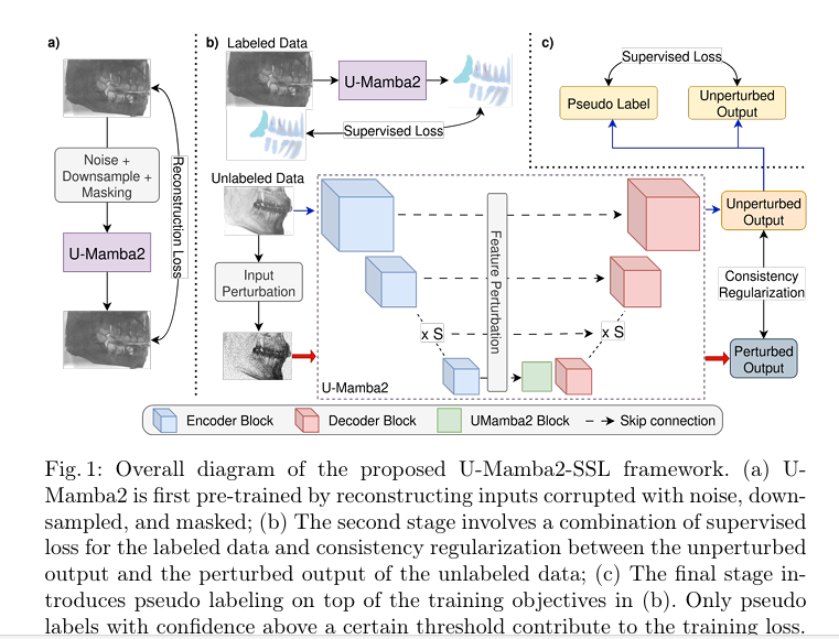
- U-Mamba2-SSL trains a Mamba2 based segmentation network in three stages, self supervised pretraining, consistency regularization, then careful pseudo labeling.
- The team had only thirty labeled CBCT volumes, split into twenty for training and ten for internal validation, while unlabeled scans were far more plentiful.
- Pretraining alone lifted the identification accuracy metric from 0.464 to 0.731, the single biggest jump in the whole recipe.
- The final scaled up model scored a 0.917 Dice coefficient and an average score of 0.789 on the hidden test set, taking first place in Task 1 of STSR 2025.
- The authors also measured how much sliding window inference speed they could trade away, cutting inference time by 53 percent for a loss of just 0.002 average score.
- Code is public on GitHub, which means the recipe is reproducible rather than just described in the abstract.
The problem hiding underneath every dental AI paper
Every automated segmentation project in dentistry runs into the same wall eventually. A cone beam CT scan of a jaw is a dense 3D volume, often hundreds of slices deep, and to train a model to separate tooth from pulp from bone from background, someone with real clinical training has to trace the boundaries of every structure by hand. The paper’s authors, Zhi Qin Tan, Xiatian Zhu, Owen Addison, and Yunpeng Li, note that this manual process demands specialized expertise and eats an enormous amount of time given how many voxels a single high resolution scan contains and how much anatomy varies from patient to patient.
That scarcity is not a minor inconvenience. It shapes the entire design of the STSR 2025 challenge, which stands for Semi supervised Teeth and Pulp Root canal Segmentation. The organizers gave competitors only thirty labeled training volumes. Everything else in the provided data was unlabeled. If you want a model that generalizes well under those conditions, you cannot simply throw more supervised training at it, because there is no more supervision to throw. You have to get useful signal out of scans nobody has annotated.
This is where semi supervised learning earns its keep. Rather than treating unlabeled data as dead weight, a semi supervised pipeline tries to extract structure from it directly, whether through self supervised pretraining, through forcing the model to behave consistently under perturbation, or through trusting the model’s own confident predictions as a rough substitute for ground truth. U-Mamba2-SSL leans on all three ideas at once, applied in a deliberate order rather than mixed together from the start.
Where these ideas actually came from
None of the three techniques in U-Mamba2-SSL were invented for this paper, and the authors are upfront about that. What is new is how they sequence and combine them for a specific anatomical target.
Reconstruction pretraining, learned from corrupted inputs
The idea of pretraining a network by asking it to repair a corrupted version of its own input goes back to denoising autoencoders and has resurfaced repeatedly, from masked autoencoders in general computer vision to self supervised pretraining of Swin transformers for 3D medical imaging. The specific recipe U-Mamba2-SSL borrows is the disruptive autoencoder, introduced by Valanarasu and colleagues, which stacks three separate corruptions, noise, downsampling, and masking, into a single pretraining objective rather than picking just one.
Consistency regularization, the smoothness assumption made concrete
Consistency training rests on a simple intuition. If two slightly different views of the same input describe the same underlying tooth or pulp voxel, a good model should assign them the same label. Ouali and colleagues formalized this for segmentation with cross consistency training, perturbing intermediate features rather than only the raw input, and that feature level perturbation is exactly what U-Mamba2-SSL adopts for its unlabeled dental scans.
Pseudo labeling, trusting the model but not blindly
Pseudo labeling traces back to Lee’s 2013 workshop paper, which proposed simply using a model’s own confident predictions on unlabeled data as if they were ground truth labels. It is popular because it needs almost no extra machinery, but it is also the riskiest of the three ideas, since a confidently wrong prediction becomes confidently wrong training data. The paper’s approach to defusing that risk, a confidence threshold and a small loss weight, is discussed in detail below.
The three stages are not interchangeable add ons. Each stage’s final checkpoint becomes the starting point for the next stage. Pretraining happens first because it needs no labels at all and gives the network a sensible starting point instead of random weights. Consistency regularization comes second because it needs a model that already produces roughly sensible outputs before its stability can be usefully measured. Pseudo labeling comes last because it needs a model good enough that its confident predictions are worth trusting even a little.
Stage one, waking the network up without any labels
In the first stage, U-Mamba2-SSL pretrains on every scan the challenge provided, labeled and unlabeled together, using the disruptive autoencoder method. Three separate corruptions get applied to the input volume before the network sees it.
Denoising asks the model to restore an image after random additive Gaussian noise has been injected into it, forcing attention to fine edges and textures. Super resolution artificially downsamples the scan with linear interpolation and asks the model to recover the higher resolution original, which requires blending local detail with broader spatial context. Masking blanks out random small cubes of the volume entirely, setting those voxels to zero, and the authors deliberately keep the cube size small relative to the scan’s spatial dimensions, reasoning that most of the useful signal in a dental CT sits in fine local detail rather than large scale structure, so discarding too much of it would defeat the purpose.
After all three corruptions are combined, the network is trained to reconstruct the clean original volume using an L1 loss. Nothing about this stage requires a single expert annotation. It is pure signal extraction from raw geometry.
Stage two, teaching the model to agree with its perturbed self
Stage two is where labeled and unlabeled data start working together in the same training loop. For each labeled scan, the model is trained the ordinary way, with a combined Dice and cross entropy loss against the ground truth. For each unlabeled scan, something more interesting happens.
The unlabeled volume passes through the model twice. First it goes through untouched, producing what the paper calls the unperturbed output. Then a perturbed version of the same volume goes through the model, producing the perturbed output. The training objective pushes those two outputs to match, measured with an L1 loss between them. If the model’s prediction shifts wildly just because the input got mildly disturbed, that mismatch becomes a training signal telling the network to be more stable.
Two kinds of perturbation feed into this. Input perturbation applies strong photometric augmentation, median filtering, Gaussian blur, Gaussian noise, brightness and contrast shifts, low resolution simulation, and sharpening, while deliberately avoiding spatial transforms like rotation or mirroring, because those would move anatomical structures rather than just changing their appearance, which would break the smoothness assumption the whole method depends on.
Feature perturbation goes a level deeper, disturbing the encoder’s internal feature maps before they reach the decoder through skip connections. The paper uses three specific mechanisms here. Random spatial dropout zeroes out entire channels with 0.5 probability, which is different from ordinary dropout because it encourages channels to become independently useful rather than co adapting. Random activation dropout samples a threshold between the 70th and 90th percentile and zeroes out any activation above it, deliberately suppressing the loudest, most confident signals so the network has to pay attention to quieter regions of the feature map too. Noise injection samples a uniform random tensor and multiplies it against the feature map before adding it back in, so the injected noise scales naturally with however active that part of the network already is.
All of this unsupervised signal gets weighted by a coefficient the paper calls omega CR, which ramps up on an exponential schedule from zero to a fixed target weight over the first fifth of training, and the proportion of unlabeled data used in each epoch increases linearly from 10 percent to 50 percent over the first two fifths of training. That schedule is a deliberate hedge. Early in training, before the model has learned anything reliable, unlabeled data is deprioritized so the network can lock onto the basic segmentation task using the labeled examples first.
Stage three, letting the model grade its own homework, carefully
Once stage two produces a model whose predictions are already reasonably stable under perturbation, the third stage adds pseudo labeling on top of the same consistency setup. For each voxel in an unlabeled scan, if the model’s predicted class confidence clears a fixed threshold, that predicted class becomes a stand in ground truth label for training. If the confidence falls short of the threshold, the voxel gets treated as background and excluded from the loss calculation entirely rather than forced into an uncertain guess.
This is a meaningfully conservative design choice. Rather than pseudo labeling every voxel and hoping errors average out, the method only pseudo labels where the model is already fairly sure, and it further limits the damage any wrong pseudo label can do by weighting the pseudo label loss term far lower than the supervised loss. The proportion of unlabeled data used per epoch again ramps up, this time from 30 percent to 50 percent over the first fifth of training in this stage.
Stage two combines a supervised loss on labeled data with a weighted consistency loss on unlabeled data.
$$L = L_S + \omega_{CR} L_{CR}$$Stage three adds a third weighted term for the pseudo label loss, which ignores the background class entirely.
$$L = L_S + \omega_{CR} L_{CR} + W_{PL} L_{PL}$$The actual numbers the team settled on give a sense of how cautious this final stage really is. The consistency weight WCR was set to 50, the pseudo label weight WPL was set to just 0.1, and the confidence threshold for accepting a pseudo label was set to 0.75. That gap between 50 and 0.1 is not an accident. It tells the model to trust the consistency signal heavily but to treat its own pseudo labels as only a light nudge, exactly the kind of caution you would want when the label source is the model itself rather than a trained clinician.
Pretraining leads to the largest leap in identification accuracy, from 0.464 to 0.731, while consistency regularization and pseudo labeling push it further to 0.738. Summarized finding from Tan, Zhu, Addison, and Li, arXiv:2509.20154
The architecture doing the actual segmentation
All three training stages sit on top of a specific network called U-Mamba2, which the same research group introduced in an earlier paper. U-Mamba2 takes the familiar U-Net encoder decoder shape and inserts Mamba2 state space blocks at the bottleneck, the narrowest point of the network where the encoder’s output feeds into the decoder.
Mamba2 itself comes from Dao and Gu’s work reframing state space models as a generalized form of attention, more efficient than a transformer’s quadratic attention while still capturing long range dependencies across a sequence, which in this case means long range spatial relationships across a 3D dental volume. The practical upside for a CBCT scan is real. These volumes are enormous, with the paper reporting a median input size of 337 by 640 by 640 voxels after resampling to the training data’s median spacing, and a transformer’s attention cost would balloon quickly at that scale. A state space block sidesteps that cost while still letting distant parts of the jaw inform each other, which matters when a tooth’s root curves well outside the field of view of any single local patch.
The full network follows seven encoder decoder stages and was implemented inside the nnU-Net framework, which handles patch based training and sliding window inference automatically. The final model carries 156 million parameters and requires roughly 6.22 trillion floating point operations per forward pass, according to the paper’s own accounting in its training configuration table.
What the experiments actually show
The team benchmarked three configurations against two baselines, plain nnU-Net and U-Mamba2 trained the ordinary supervised way with no semi supervised tricks. Four metrics get tracked. Dice similarity coefficient measures region overlap. Normalized surface distance measures how close predicted boundaries sit to the true boundaries. Mean intersection over union is another overlap measure. Identification accuracy, the metric that moves the most across these experiments, measures the average percentage of anatomical classes per image that clear an IoU above 0.5, which effectively asks whether the model correctly identifies each individual tooth and pulp structure rather than just getting the overall pixel overlap roughly right.
| Method | Pretrain | Consistency reg | Pseudo label | DSC | NSD | mIoU | IA | Average |
|---|---|---|---|---|---|---|---|---|
| nnU-Net baseline | No | No | No | 0.963 | 0.997 | 0.928 | 0.286 | 0.794 |
| U-Mamba2 baseline | No | No | No | 0.965 | 0.998 | 0.930 | 0.464 | 0.839 |
| U-Mamba2-SSL | Yes | No | No | 0.967 | 0.998 | 0.937 | 0.731 | 0.908 |
| U-Mamba2-SSL | Yes | Yes | No | 0.967 | 0.999 | 0.935 | 0.736 | 0.910 |
| U-Mamba2-SSL | Yes | Yes | Yes | 0.967 | 0.999 | 0.935 | 0.738 | 0.910 |
The most interesting story in that table is how little Dice, surface distance, and mean IoU move across every configuration, all hovering close to 0.96 or higher even for the plain nnU-Net baseline, while identification accuracy swings from 0.286 all the way to 0.738. That gap tells you something clinically relevant. A model can look nearly perfect on average overlap metrics while still routinely missing or merging individual small anatomical structures such as a thin pulp canal, and identification accuracy is the metric that actually catches that failure mode. Pretraining alone accounts for the overwhelming majority of the improvement, lifting identification accuracy from 0.464 to 0.731, while consistency regularization and pseudo labeling add smaller but real gains on top, from 0.731 to 0.738.
It is worth being direct about what this table does and does not prove. It shows that reconstruction pretraining does most of the heavy lifting in this particular recipe, at least by identification accuracy. Consistency regularization and pseudo labeling contribute real but comparatively modest additional gains on the same validation set. None of that guarantees the same ranking of importance would hold on a different dataset, a different anatomical target, or a different labeled to unlabeled ratio, and the paper does not claim otherwise.
For the actual challenge submission, the team scaled up their recipe considerably, training on all available data for 1000 epochs with a larger 160 by 256 by 256 input patch, and applying test time augmentation with mirroring along the anterior posterior and left right axes during inference. That scaled up model reached a DSC of 0.969, an NSD of 0.998, an mIoU of 0.940, and an IA of 0.806 on the validation set. On the hidden test set, the numbers that actually decided the challenge ranking, it scored a DSC of 0.917, an NSD of 0.882, an mIoU of 0.948, and an IA of 0.577, for an average score of 0.789, which was enough to take first place in Task 1 of the STSR 2025 challenge.
That test set drop, particularly identification accuracy falling from 0.806 on the internal validation set to 0.577 on the hidden test set, is a useful reminder that even a winning entry does not fully close the gap between validation performance and truly unseen data. The authors do not dwell on this gap in their discussion, but it is visible directly in their own reported numbers.
Squeezing out inference time without giving up much accuracy
Because the STSR 2025 challenge also scored algorithm runtime and memory use, the team ran a separate set of experiments purely on speed, described in the paper’s supplementary material. Sliding window inference has two knobs that trade accuracy for time, the tile size, which controls how much the sliding window steps overlap, and the choice of which spatial axes get mirrored for test time augmentation.
Since most voxels in a CBCT scan belong to the background class, the authors found that raising the tile size to 0.9 cut inference time by 53 percent while only costing 0.002 average score, a genuinely favorable trade. On the mirroring axes, using all three axes gave the best raw performance but at a real time cost, while mirroring only the anterior posterior and left right axes, labeled ‘1,2’ in the paper’s axis notation, delivered a strong average score with an inference time of just 17.08 seconds.
The clinical translation gap
Everything above describes what happened on a research benchmark, and it is worth being honest about the distance between that benchmark and an actual dental clinic. The STSR 2025 challenge used a curated dataset with thirty labeled training scans and a separate hidden test set assembled by the challenge organizers. That is a controlled research setting, not the messy variability of scanners, acquisition protocols, patient positioning, and image artifacts a model would meet in routine practice across different clinics and different CBCT machine manufacturers.
The paper itself flags a related limitation. Its dataset mixes full field of view CBCTs with limited field of view CBCTs, and the authors note their model produces more false positives around image edges specifically on the limited field of view scans, exactly the kind of scan variability a real clinical deployment would need to handle robustly rather than as an edge case. There is also no reported evaluation against inter observer variability among human experts, which is the usual yardstick for judging whether an AI system’s disagreements with one annotator fall inside the normal range of disagreement between two human experts.
None of this diminishes what the paper demonstrates technically. It does mean that a strong result on a hidden challenge test set is a research milestone, not a regulatory clearance, and the authors themselves frame their contribution as a challenge submission rather than a clinically validated tool.
Where this line of work could go next
The authors point to two concrete directions for future work, and both are grounded in limitations they observed directly rather than speculative wish lists. First, because full field of view and limited field of view CBCTs carry genuinely different information and image properties, they suggest future systems should use data processing and augmentation strategies tailored to each scan type rather than treating all CBCTs identically. Second, since the anatomically relevant foreground classes typically occupy only a small region of interest inside a much larger volume that is otherwise background, they suggest future work could avoid wasting computation and training time on background heavy regions and instead let the model concentrate its capacity on the region of interest.
Beyond the paper’s own stated directions, the general recipe, self supervised reconstruction pretraining followed by consistency regularization followed by cautious pseudo labeling, is not inherently specific to teeth and pulp. The same three stage structure could plausibly transfer to other 3D medical segmentation tasks that share the same core constraint the authors started with, a small pool of expensive expert labeled volumes sitting next to a much larger pool of unlabeled scans, which describes a great many corners of radiology beyond dentistry.
Honest limitations
A few limitations are worth stating plainly, beyond the two the authors raise themselves. The labeled training set was small, twenty volumes for actual training and ten held back for internal validation, which is a narrow base from which to draw strong generalization claims even with a large unlabeled pool supporting it. The paper reports strong metrics on both the internal validation set and the hidden test set, but the identification accuracy metric specifically dropped from 0.806 on validation to 0.577 on the hidden test set for the final challenge model, a meaningful gap that deserves attention rather than being smoothed over.
The paper also does not report results broken down by tooth type, root canal complexity, or patient demographic group, so it is not possible from this paper alone to know whether performance is uniform across different anatomical presentations or whether certain harder cases, such as heavily calcified canals or atypical root morphology, are systematically underperforming. As a preprint tied to a challenge submission rather than a peer reviewed clinical validation study, its claims should be read as a strong technical result on a specific benchmark, not as evidence of readiness for clinical deployment.
Read the source material
The full method, ablation tables, and supplementary inference speed experiments are available directly from the authors.
A complete PyTorch implementation of the core ideas
What follows is a runnable, simplified reimplementation of the three stage recipe, written to be readable rather than to match every last detail of the authors’ nnU-Net integration. It uses a small 3D U-Net style backbone in place of the full U-Mamba2 network so it can run a smoke test on dummy data without requiring the Mamba2 kernels, but the training logic for the disruptive autoencoder pretraining, the consistency regularization with feature perturbation, and the confidence thresholded pseudo labeling all follow the paper’s description directly.
Bringing it together
The core achievement here is not a single new architecture or a single new loss function. It is a demonstration that three well known ideas, self supervised reconstruction pretraining, feature level consistency regularization, and cautious confidence gated pseudo labeling, can be chained together with careful scheduling to squeeze real performance out of a labeled dataset with only thirty scans, when Mamba2 gives the underlying network enough capacity to model long range spatial structure efficiently.
There is a real conceptual shift buried in how the paper reports its own results, too. The team did not just optimize for Dice coefficient, a metric where their gains over a plain U-Mamba2 baseline were modest, moving from 0.965 to 0.967. They paid attention to identification accuracy, the metric that actually captures whether individual anatomical structures get correctly recognized as distinct entities, and that is where the semi supervised recipe delivered its real value, climbing from 0.464 to 0.738 on the validation set. That distinction matters for anyone evaluating segmentation models generally, since overall overlap metrics can mask exactly the kind of small structure failures that matter most in a clinical context.
The three stage recipe also seems genuinely transferable beyond dentistry. Nothing about disruptive autoencoder pretraining, feature perturbed consistency regularization, or confidence thresholded pseudo labeling is specific to teeth, pulp, or even to CBCT imaging as a modality. Any 3D medical segmentation task built around a small expert labeled dataset sitting next to a larger unlabeled pool, which describes a large share of specialized radiology problems, could plausibly borrow this exact staged approach.
At the same time, the honest remaining limitations deserve equal weight to the headline first place result. Thirty labeled volumes is a small foundation, the identification accuracy metric dropped noticeably between the internal validation set and the hidden test set, and the dataset’s mix of full and limited field of view scans already exposed a specific failure mode around image edges that the authors themselves flagged rather than glossed over. Those are the kinds of details that separate a paper worth reading closely from a paper worth taking at face value.
Taken as a whole, U-Mamba2-SSL reads less like a single clever trick and more like a disciplined engineering exercise in extracting every bit of usable signal from a genuinely data scarce medical imaging problem, backed by public code that lets anyone check the claims directly rather than trusting the abstract alone.
Frequently asked questions
What exactly is U-Mamba2-SSL?
It is a semi supervised training framework built on top of the U-Mamba2 segmentation network, developed by researchers at King’s College London and the University of Surrey for the STSR 2025 dental imaging challenge. It trains in three stages, self supervised pretraining, consistency regularization, and confidence thresholded pseudo labeling, to make use of unlabeled CBCT scans alongside a small labeled dataset.
How many labeled scans did the researchers actually have?
Only thirty labeled CBCT volumes were provided by the challenge, which the team split into twenty for training and ten for internal validation. The unlabeled pool of scans was significantly larger, which is exactly the imbalance semi supervised learning is designed to address.
What is a disruptive autoencoder in this context?
It is a self supervised pretraining method that combines three corruption tasks, denoising a noisy input, recovering detail lost through downsampling, and filling in masked out cubes of the volume, all trained together with a single reconstruction loss before any labeled training begins.
Did this model actually win a competition?
Yes. The scaled up version of U-Mamba2-SSL scored an average of 0.789 and a Dice coefficient of 0.917 on the hidden test set, which secured first place in Task 1 of the STSR 2025 challenge, according to the paper’s reported results.
Is U-Mamba2-SSL ready to be used in a dental clinic?
No. This is a research model evaluated on a specific academic challenge dataset. It has not gone through clinical validation, regulatory review, or testing across the range of scanners and patient populations a real deployment would require. Any dental imaging AI questions relevant to actual patient care should go to a licensed dentist or radiologist.
What is Mamba2 and why does it matter for a dental CT scan?
Mamba2 is a state space model architecture from Dao and Gu that captures long range dependencies more efficiently than transformer style attention. Inserted at the bottleneck of U-Mamba2, it lets the network relate distant parts of a large 3D dental volume, such as a curving tooth root, without the steep computational cost a full attention mechanism would carry at that scale.
Academic citation. Tan, Z. Q., Zhu, X., Addison, O., and Li, Y. U-Mamba2-SSL for Semi Supervised Tooth and Pulp Segmentation in CBCT. arXiv:2509.20154, 2025.
This analysis is based on the published paper and an independent evaluation of its claims.