
Key points
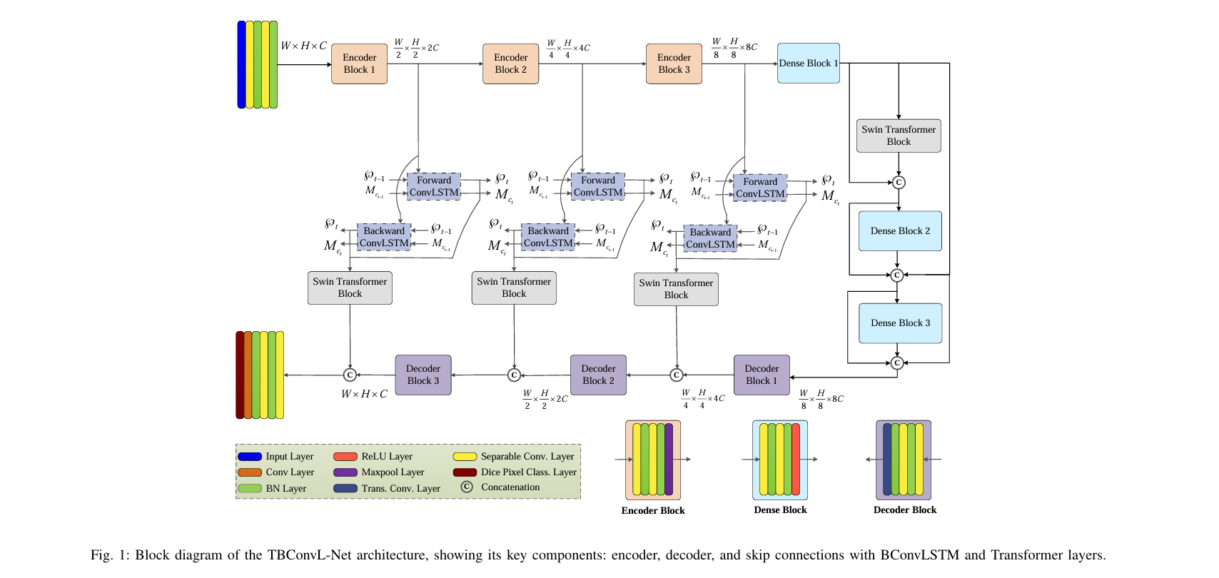
- TBConvL-Net combines a CNN encoder decoder with bidirectional ConvLSTM and lightweight Swin Transformer blocks placed specifically inside the skip connections.
- It reports the best score on every listed metric across all ten datasets tested, including a Jaccard index of 91.65 percent on ISIC 2018 skin lesions and 92.93 percent on TCIA brain tumor segmentation.
- The model runs with only 9.6 million parameters and a 19.1 millisecond inference time, notably lighter than Swin-Unet’s 27.3 million parameters and 34.8 milliseconds.
- The paper’s own ablation study shows that placing the Swin Transformer in the wrong location actually hurts performance below even the simplest baseline, making placement, not just presence, the deciding factor.
- Every baseline comparison number in the results tables was copied from the original publishing papers rather than rerun by the authors under identical conditions, a detail worth knowing before treating the head to head margins as precise.
The specific limitation this paper is targeting
Accurately outlining a lesion or pathology in a medical image, a mole on skin, a nodule on a thyroid ultrasound, a tumor on a brain MRI, is genuinely difficult work, and relying purely on expert visual judgment can be slow and subject to variation based on individual clinical experience. Automated segmentation exists to help with exactly that, and convolutional neural networks have been the default tool for the job for years, with U-Net and its many variants becoming close to a standard starting point across the field.
The authors point to a specific structural weakness in that default approach. Convolutional operations are inherently local, a small kernel only looks at a small neighborhood of pixels, which means a plain CNN struggles to capture long range relationships across an image, and its learned filters stay fixed once training ends regardless of what a new input actually contains. Vision transformers address the long range dependency problem directly through self attention, and models like TransUNet were the first to combine CNN and transformer components for medical segmentation specifically. But transformers bring their own tradeoffs, they tend to need large training sets to work well, and a plain self attention layer applied at a single token granularity can struggle to capture how different channels of information relate to each other at different scales, which matters when the pathology you are trying to outline varies enormously in size and shape from one patient to the next.
What TBConvL-Net actually adds
TBConvL-Net keeps a fairly conventional CNN encoder decoder backbone, built from depth wise separable convolutions rather than standard convolutions to cut computational cost while preserving feature quality, and adds densely connected blocks so that feature maps from earlier layers stay available to later ones rather than being discarded. The real contribution sits in how the skip connections between the encoder and decoder are handled. Rather than passing encoder features straight across to the decoder the way standard U-Net does, TBConvL-Net routes them through a combination of bidirectional ConvLSTM, shortened to BConvLSTM, and a lightweight Swin Transformer block.
The reasoning behind that specific combination is worth spelling out. Encoder features carry high resolution, fine grained spatial detail. Decoder features carry higher level semantic understanding built up over the network’s depth. Bridging that gap well, transferring rich contextual information from encoder to decoder without losing either the fine detail or the semantic understanding, is where the authors argue standard skip connections fall short. BConvLSTM handles the temporal side of that bridge, treating the relationship between encoder and decoder features somewhat like a sequence problem, with a forward pass and a backward pass each capturing different directional dependencies. The Swin Transformer block handles the spatial side, using shifted window based self attention to model long range dependencies and dynamic attention across the image, at linear rather than quadratic computational cost relative to image size, since the paper specifically flags standard self attention’s quadratic complexity as a barrier to using transformers in dense pixel level prediction tasks like segmentation.
Inside the ConvLSTM block
The ConvLSTM mechanism follows the same conceptual structure as a standard LSTM, a memory cell, an input gate, a forget gate, and an output gate, but replaces the usual fully connected operations with convolutional ones, which lets the network preserve spatial correlation in the data rather than flattening it away.
Here $\otimes$ denotes a Hadamard, or element wise, operation and $\circledast$ denotes a convolution, $\Im_t$ and $\wp_t$ are the input and hidden state tensors, and $\beta_{M_c}$ is the memory cell’s bias term. The forget, input, and output gates each follow a similar structure, each gated by a sigmoid function and each combining convolutions over the current input and the previous hidden state.
The bidirectional version processes the sequence of features in both a forward direction and a backward direction, then combines the two using a hyperbolic tangent function, which the authors state helps the network capture complex relationships between forward and backward dependencies in the input data that a single directional pass would miss.
Inside the lightweight Swin Transformer block
Rather than applying self attention globally across an entire image, which scales quadratically with the number of image patches and becomes prohibitively expensive for anything but small inputs, the Swin Transformer restricts attention to local, non overlapping windows of patches, and alternates between regular and shifted window positions across consecutive blocks so that information can still eventually propagate across the whole image. The computational cost comparison the authors cite makes the motivation concrete, a standard multihead self attention module costs on the order of $4(h \times w)d^2 + 2(h \times w)^2 d$ operations, quadratic in the number of patches, while the shifted window version costs $4(h \times w)d^2 + 2N^2(h \times w)d$, linear for a fixed window size $N$.
Each transformer block pairs a regular windowed self attention module with a shifted windowed one across two consecutive stages, each followed by layer normalization and a multilayer perceptron, with the outputs concatenated at each step rather than simply replaced, preserving information from earlier processing stages as the features move through the block.
A composite loss function built around boundary agreement
Rather than training purely on a single loss function, TBConvL-Net combines three, Dice loss, Jaccard loss, and a dedicated boundary loss, into a single weighted total.
The reasoning given for combining Dice and Jaccard specifically is that Dice loss rewards getting the overall size and shape of a predicted region right, even allowing for a slight positional shift, while Jaccard loss is stricter about the predicted region actually overlapping the correct location. The boundary loss term is different in kind, it works directly on the distance between the predicted segmentation’s boundary and the ground truth boundary, based on earlier work on boundary loss for highly imbalanced segmentation tasks, rather than measuring overlap at all. In training, the Dice and Jaccard weights were held at 1, while the boundary loss weight started at 1 and was gradually reduced by 0.01 per epoch down to a floor of 0.01, a schedule the authors describe as moderating the boundary term’s influence so it remains meaningful without dominating the overall optimization.
Ten datasets, seven modalities, and how uneven they really are
The breadth of testing here is genuinely unusual for a single architecture paper. ISIC 2016, 2017, and 2018 cover skin lesion segmentation in dermoscopic optical images. DDTI covers thyroid nodule segmentation in ultrasound. BUSI covers breast lesion segmentation in ultrasound, specifically in patients aged 25 to 75. MoNuSeg covers nuclei segmentation in histopathological whole slide microscopy images. MC covers chest X-ray lung segmentation. IDRiD covers optic disc segmentation in fundus photographs. Fluorescent Neuronal Cells covers cell segmentation in fluorescence microscopy. TCIA covers brain tumor segmentation in MRI.
What is easy to miss in a results table full of strong percentages is how small some of these datasets actually are. MoNuSeg totals just 44 images, 30 for training and 14 for testing. IDRiD totals 81 images. MC totals 138. Fluorescent Neuronal Cells totals 353. DDTI and BUSI do not even have a dedicated test set at all, the authors evaluated performance on those two using five fold cross validation instead, specifically because a separate held out test partition was not available.
| Dataset | Modality | Total images | Evaluation approach |
|---|---|---|---|
| ISIC 2018 | Optical, skin lesions | 3594 | Fixed train and test split |
| DDTI | Ultrasound, thyroid nodules | 637 | Five fold cross validation, no separate test set |
| BUSI | Ultrasound, breast lesions | 780 | Five fold cross validation, no separate test set |
| MoNuSeg | Whole slide microscopy, nuclei | 44 | Fixed train and test split |
| MC | X-ray, chest | 138 | Fixed train and test split |
| IDRiD | Fundus, optic disc | 81 | Fixed train and test split |
| Fluorescent Neuronal Cells | Fluorescence microscopy | 353 | Fixed train and test split |
| TCIA | MRI, brain tumor | 1369 | Fixed train and test split |
What the reported numbers actually show
TBConvL-Net reports the top score on every single metric across every one of the ten datasets in its comparison tables, which is a remarkably clean sweep. On the ISIC skin lesion datasets, it reached a Jaccard index of 91.65 percent on ISIC 2018, 84.8 percent on ISIC 2017, and 89.47 percent on ISIC 2016, ahead of Swin-Unet, ARU-GD, FAT-Net, and a long list of other published methods on each. On the DDTI thyroid nodule dataset, it reached 88.70 percent Jaccard, edging out the next closest listed competitor, N-Net, at 88.46 percent. On BUSI breast lesion segmentation, the gap was much larger, 91.97 percent Jaccard against Swin-Unet’s 77.16 percent. On brain tumor segmentation using TCIA, it reached 92.93 percent Jaccard against a plain U-Net’s 86.15 percent.
| Dataset | Best listed competitor | Competitor Jaccard | TBConvL-Net Jaccard |
|---|---|---|---|
| ISIC 2018 | ARU-GD | 84.55 | 91.65 |
| DDTI | N-Net | 88.46 | 88.70 |
| BUSI | Swin-Unet | 77.16 | 91.97 |
| MoNuSeg | BCDU-Net and c-ResUnet, tied | 66.61 | 76.07 |
| IDRiD | ARU-GD | 91.59 | 95.65 |
| TCIA brain tumor | Swin-Unet | 83.46 | 92.93 |
What the transformer placement ablation actually reveals
The most informative part of the paper is not the final comparison table, it is the ablation study on where exactly to put the Swin Transformer. Starting from a simple bidirectional ConvLSTM U-Net as a baseline, which reached 79.20 percent Jaccard on ISIC 2017, the authors first swapped in depth wise separable convolutions, which alone lifted performance to 80.14 percent. From there, they tested inserting the Swin Transformer at four different locations. Placing it between the dense layers of the network actually reduced performance to 78.61 percent, below even the separable convolution baseline without any transformer at all. Placing it after every pooling layer in the decoder brought performance to 81.53 percent. Placing it between the skip connections reached 81.70 percent. Only when placed between both the skip connections and the dense layers simultaneously, the configuration the final model actually uses, did performance reach the reported peak of 82.78 percent Jaccard.
What the loss function ablation shows
On the DDTI thyroid dataset, the authors tested Dice, Jaccard, and boundary loss individually and in combination. Individually, boundary loss alone performed worst on ISIC 2017 at only 63.06 percent Jaccard, while Dice loss alone reached 78.72 percent. Combining Dice and Jaccard together actually underperformed Dice alone in one comparison, reaching only 67.26 percent on ISIC 2017 in one particular pairing, a reminder that loss function combinations do not always compose in the direction you would expect. The full three way combination of Dice, Jaccard, and boundary loss reached the best result on both datasets tested, 83.91 percent Jaccard on ISIC 2017 and 86.06 percent on DDTI, which is why the final model uses all three together rather than any single loss or two way pairing.
What transfer learning added, and where it did not help
A third ablation tested whether pretraining on one dataset before fine tuning on another would help, transferring learned weights between related modalities, for instance training first on ISIC 2017 before fine tuning on ISIC 2016, or training first on BUSI before fine tuning on DDTI. Across most datasets, transfer learning produced a real improvement, lifting BUSI’s Jaccard from 85.95 to 91.97 percent and DDTI’s from 86.06 to 88.70 percent. On two datasets specifically, MC chest X-rays and IDRiD optic disc images, the authors report that the model already reached its best performance without transfer learning at all, with MC actually showing an essentially flat result, 97.88 percent Jaccard without transfer learning against 97.90 percent with it, a difference small enough to fall within normal run to run variation rather than a meaningful gain.
The parameter count and speed comparison
TBConvL-Net reports 9.6 million parameters, 15.5 billion floating point operations, and a 19.1 millisecond inference time. Every comparison model listed in the complexity table is heavier, U-Net at 23.6 million parameters and 28.9 milliseconds, Swin-Unet at 27.3 million parameters, 37.0 billion FLOPs, and 34.8 milliseconds, nearly double TBConvL-Net’s inference time for a model built entirely around global self attention. That is a genuinely favorable tradeoff on paper, a lighter, faster model reporting higher accuracy across the board, though it is worth remembering that all of these baseline complexity numbers, like the accuracy numbers, come from the authors’ own measurement of publicly available implementations rather than a fully independent third party benchmark.
Clinical translation gap
A detail buried in the methodology section deserves more attention than it usually gets in a summary of results. The authors state plainly that given the large number of comparison methods and the unavailability of many of their original implementations, it was not feasible to reimplement, retrain, or rerun them, so the comparison numbers in every results table were copied directly from the original publishing papers rather than reproduced by the authors themselves under one shared, controlled experimental setup. That is a common and understandable practice in a field this crowded, but it means the reported margins between TBConvL-Net and its competitors reflect differences that could partly stem from different preprocessing choices, different data splits, or different training budgets across the original papers, not solely from architectural superiority. The authors are transparent about this limitation themselves, and it is worth taking at face value rather than glossing over when reading the comparison tables.
There is also a real gap between what these ten datasets represent and what a functioning clinical tool would need to demonstrate. Several of the smallest datasets here, MoNuSeg at 44 total images, IDRiD at 81, MC at 138, are small enough that a handful of difficult or unusual cases in the test set could meaningfully swing the reported metrics, and two of the datasets, DDTI and BUSI, were evaluated with cross validation rather than an independent test set specifically because no separate test partition existed at all. None of the ten datasets represent a prospective clinical deployment, they are retrospective, curated research collections, several drawn from single institutions or single public archives, and the paper does not report results on external validation cohorts collected under different imaging equipment or different patient populations than the original benchmark data.
It is also worth being precise about what a Jaccard index or Dice score in the low to high nineties actually tells a clinician. These are geometric overlap measures between a predicted mask and a ground truth mask drawn by whoever annotated the original dataset. They say nothing directly about how a clinician would use the output, as a fully automated first pass, as a starting point for manual correction, or as a second opinion alongside their own reading, and nothing in this paper tests that downstream question.
Clinical and technical limitations worth sitting with
A few specific points are worth naming directly. The comparison tables mix results generated by the authors’ own experiments with numbers copied wholesale from other papers, and the authors themselves acknowledge this was a practical necessity rather than an ideal experimental design, which means the exact percentage gaps reported against competing methods should be read as approximate rather than precise. Several of the ten datasets are genuinely small by deep learning standards, and two lack an independent test set entirely, relying on cross validation instead, a reasonable substitute but not equivalent to a truly held out evaluation.
The paper also reports what appears to be a single training run per dataset configuration rather than repeated runs with confidence intervals, so small differences between ablation configurations, some separated by less than a single percentage point, deserve some skepticism about how consistently they would replicate. And while the model’s efficiency gains, fewer parameters, fewer FLOPs, faster inference, are reported clearly and consistently across every comparison, none of the ten datasets or evaluation protocols involve anything resembling a real time clinical deployment scenario, so the practical value of that speed advantage outside a research benchmark context remains untested here.
Why this still matters despite the caveats
Strip away the clinical translation question, and the ablation study on transformer placement is a genuinely valuable piece of engineering knowledge on its own. Most papers that add a transformer component to a CNN architecture report only the final configuration’s performance, leaving the reader to assume that placement was obvious or that any reasonable placement would have worked about as well. This paper shows concretely that it would not have, that the specific choice of routing the Swin Transformer through both the skip connections and the dense layers together was doing meaningfully more work than putting it almost anywhere else in the network. That is useful, transferable knowledge for anyone designing a hybrid CNN transformer segmentation model, independent of whether TBConvL-Net’s exact headline numbers hold up under a fully independent, third party reevaluation.
Full conclusion
The core contribution here is a specific, carefully ablated recipe for combining CNN encoder decoder features with a temporal, bidirectional ConvLSTM path and a spatial, windowed self attention path, routed specifically through the skip connections rather than scattered elsewhere in the network. The breadth of testing, seven modalities and ten datasets, is a genuine strength relative to the more common single dataset architecture paper, and the placement and loss function ablations give real, granular insight into which design choices are actually earning their keep rather than presenting the final model as an unexamined black box.
The conceptual lesson worth remembering is narrower than the clean sweep of best scores across every table might suggest. This is not evidence that hybrid CNN transformer architectures are now a solved recipe for medical segmentation. It is evidence that where you place a transformer inside a network matters as much as whether you use one at all, that a wrongly placed attention block can actively hurt performance, and that a composite loss combining overlap based and boundary based terms outperforms any single loss function tested here.
Whether the exact reported margins over competing methods would hold up under a fully independent, apples to apples reevaluation is a genuinely open question, given the authors’ own disclosure that comparison numbers were copied from original papers rather than reproduced under one shared protocol. That is not a criticism unique to this paper, it reflects a real practical constraint common across a crowded research field, but it is a meaningful caveat for anyone treating the specific percentage point gaps as precise rather than indicative.
The honest remaining limitations are the ones already laid out above and should not be softened. Several of the ten datasets are small enough that individual difficult cases could meaningfully shift reported metrics. Two datasets relied on cross validation rather than an independent test set. And nothing in this paper tests how the model would perform on external data collected under different imaging equipment or different patient populations than its original benchmark sources.
Put simply, TBConvL-Net is a well ablated, broadly tested architecture contribution that offers real, specific engineering insight, particularly around transformer placement, and it is not, and does not claim to be, a validated clinical segmentation tool. Reading it as the former rather than the latter is the accurate way to take both its genuine strengths and its real limits seriously at the same time.
Reference implementation in PyTorch
The code below is an independent, simplified implementation of the core TBConvL-Net idea, a CNN encoder decoder whose skip connections are routed through a bidirectional ConvLSTM and a lightweight windowed self attention block, plus the paper’s composite Dice, Jaccard, and boundary loss. It is not the authors’ original code, which the paper does not publish a link to, and it uses a compact 2D backbone rather than the paper’s full multi stage network to keep the example runnable and focused on the skip connection design that is the actual contribution of this paper.
# tbconvl_net_reference.py
# Independent reference implementation of the core TBConvL-Net idea,
# a CNN encoder decoder whose skip connections route through a
# bidirectional ConvLSTM and a lightweight windowed self attention
# block, plus the paper's composite Dice, Jaccard, and boundary loss.

import torch
import torch.nn as nn
import torch.nn.functional as F


class ConvLSTMCell(nn.Module):
    """A single direction ConvLSTM cell, Equations 8 through 12.
    Replaces the fully connected gates of a standard LSTM with
    convolutions so spatial structure is preserved."""

    def __init__(self, channels, hidden_channels, kernel_size=3):
        super().__init__()
        padding = kernel_size // 2
        self.hidden_channels = hidden_channels
        # one combined conv producing all four gates at once
        self.gates = nn.Conv2d(
            channels + hidden_channels, hidden_channels * 4,
            kernel_size=kernel_size, padding=padding
        )

    def forward(self, x, hidden_state):
        h_prev, c_prev = hidden_state
        combined = torch.cat([x, h_prev], dim=1)
        gates = self.gates(combined)
        i, f, o, g = torch.chunk(gates, 4, dim=1)

        i = torch.sigmoid(i)
        f = torch.sigmoid(f)
        o = torch.sigmoid(o)
        g = torch.tanh(g)

        c_next = f * c_prev + i * g
        h_next = o * torch.tanh(c_next)
        return h_next, c_next

    def init_hidden(self, batch_size, spatial_size, device):
        h, w = spatial_size
        return (
            torch.zeros(batch_size, self.hidden_channels, h, w, device=device),
            torch.zeros(batch_size, self.hidden_channels, h, w, device=device),
        )


class BConvLSTM(nn.Module):
    """Bidirectional ConvLSTM, Equation 13. Runs a forward and a
    backward ConvLSTM cell over a short sequence of feature maps
    built from the encoder and decoder features, then combines them
    with a tanh nonlinearity."""

    def __init__(self, channels, hidden_channels=None):
        super().__init__()
        hidden_channels = hidden_channels or channels
        self.forward_cell = ConvLSTMCell(channels, hidden_channels)
        self.backward_cell = ConvLSTMCell(channels, hidden_channels)
        self.out_conv = nn.Conv2d(hidden_channels * 2, channels, kernel_size=1)

    def forward(self, sequence):
        # sequence is a list of feature maps, shape batch, channels, h, w
        b, _, h, w = sequence[0].shape
        device = sequence[0].device

        fwd_state = self.forward_cell.init_hidden(b, (h, w), device)
        for step in sequence:
            fwd_state = self.forward_cell(step, fwd_state)

        bwd_state = self.backward_cell.init_hidden(b, (h, w), device)
        for step in reversed(sequence):
            bwd_state = self.backward_cell(step, bwd_state)

        combined = torch.cat([fwd_state[0], bwd_state[0]], dim=1)
        return torch.tanh(self.out_conv(combined))


class LightweightWindowAttention(nn.Module):
    """A simplified stand in for the Swin Transformer block, restricting
    self attention to local windows to keep cost linear in image size
    rather than quadratic, following the motivation in Equations 14
    and 15."""

    def __init__(self, channels, window_size=4, num_heads=4):
        super().__init__()
        self.window_size = window_size
        self.norm = nn.LayerNorm(channels)
        self.attn = nn.MultiheadAttention(channels, num_heads, batch_first=True)
        self.mlp = nn.Sequential(
            nn.Linear(channels, channels * 2), nn.GELU(), nn.Linear(channels * 2, channels)
        )

    def forward(self, x):
        b, c, h, w = x.shape
        ws = self.window_size
        # pad so height and width divide evenly into windows
        pad_h = (ws - h % ws) % ws
        pad_w = (ws - w % ws) % ws
        x_padded = F.pad(x, (0, pad_w, 0, pad_h))
        _, _, hp, wp = x_padded.shape

        # reshape into non overlapping windows, each treated as a mini sequence
        windows = x_padded.unfold(2, ws, ws).unfold(3, ws, ws)
        n_wh, n_ww = windows.shape[2], windows.shape[3]
        windows = windows.contiguous().view(b, c, n_wh * n_ww, ws * ws)
        windows = windows.permute(0, 2, 3, 1).reshape(b * n_wh * n_ww, ws * ws, c)

        normed = self.norm(windows)
        attn_out, _ = self.attn(normed, normed, normed)
        windows = windows + attn_out
        windows = windows + self.mlp(self.norm(windows))

        # fold windows back into a full feature map and remove padding
        windows = windows.view(b, n_wh * n_ww, ws * ws, c).permute(0, 3, 1, 2)
        windows = windows.view(b, c, n_wh, n_ww, ws, ws)
        out = windows.permute(0, 1, 2, 4, 3, 5).reshape(b, c, hp, wp)
        return out[:, :, :h, :w]


class SkipFusion(nn.Module):
    """Fuses an encoder skip feature with the current decoder feature
    using BConvLSTM for the temporal path and windowed attention for
    the spatial path, then concatenates both, mirroring how skip
    connections are handled in Section 3.B of the paper."""

    def __init__(self, channels):
        super().__init__()
        self.bconvlstm = BConvLSTM(channels)
        self.window_attn = LightweightWindowAttention(channels)
        self.fuse = nn.Conv2d(channels * 2, channels, kernel_size=1)

    def forward(self, encoder_feat, decoder_feat):
        temporal = self.bconvlstm([encoder_feat, decoder_feat])
        spatial = self.window_attn(encoder_feat)
        fused = torch.cat([temporal, spatial], dim=1)
        return self.fuse(fused)


class TBConvLNetLite(nn.Module):
    """A compact stand in for the full TBConvL-Net pipeline, with a
    three stage encoder decoder and SkipFusion modules bridging each
    resolution level."""

    def __init__(self, in_channels=3, num_classes=1, base=16):
        super().__init__()
        self.enc1 = nn.Sequential(nn.Conv2d(in_channels, base, 3, padding=1), nn.ReLU(inplace=True))
        self.enc2 = nn.Sequential(nn.Conv2d(base, base * 2, 3, stride=2, padding=1), nn.ReLU(inplace=True))
        self.enc3 = nn.Sequential(nn.Conv2d(base * 2, base * 4, 3, stride=2, padding=1), nn.ReLU(inplace=True))

        self.skip2 = SkipFusion(base * 2)
        self.skip1 = SkipFusion(base)

        self.dec2 = nn.Sequential(nn.ConvTranspose2d(base * 4, base * 2, 2, stride=2), nn.ReLU(inplace=True))
        self.dec1 = nn.Sequential(nn.ConvTranspose2d(base * 2, base, 2, stride=2), nn.ReLU(inplace=True))

        self.out_conv = nn.Conv2d(base, num_classes, kernel_size=1)

    def forward(self, x):
        e1 = self.enc1(x)
        e2 = self.enc2(e1)
        e3 = self.enc3(e2)

        d2 = self.dec2(e3)
        d2 = self.skip2(e2, d2)
        d1 = self.dec1(d2)
        d1 = self.skip1(e1, d1)

        return self.out_conv(d1)


def dice_loss(logits, targets, eps=1e-6):
    """Equation 20, simplified for binary segmentation."""
    probs = torch.sigmoid(logits)
    intersection = (probs * targets).sum(dim=(2, 3))
    union = (probs ** 2).sum(dim=(2, 3)) + (targets ** 2).sum(dim=(2, 3))
    dice = (2 * intersection + eps) / (union + eps)
    return 1 - dice.mean()


def jaccard_loss(logits, targets, eps=1e-6):
    """Equation 21, simplified to the standard soft IoU form."""
    probs = torch.sigmoid(logits)
    intersection = (probs * targets).sum(dim=(2, 3))
    union = probs.sum(dim=(2, 3)) + targets.sum(dim=(2, 3)) - intersection
    iou = (intersection + eps) / (union + eps)
    return 1 - iou.mean()


def boundary_loss(logits, distance_map):
    """A simplified stand in for Equation 25. Expects a precomputed
    signed distance map of the ground truth boundary and weights the
    predicted probability map by that distance, penalising confident
    predictions far from the true boundary."""
    probs = torch.sigmoid(logits)
    return (distance_map * probs).mean()


def composite_loss(logits, targets, distance_map, lambda_d=1.0, lambda_j=1.0, lambda_b=0.5):
    """Equation 26, the weighted sum of Dice, Jaccard, and boundary loss."""
    return (
        lambda_d * dice_loss(logits, targets)
        + lambda_j * jaccard_loss(logits, targets)
        + lambda_b * boundary_loss(logits, distance_map)
    )


def run_smoke_test():
    """Runs a short training loop on random dummy images to confirm the
    model, skip fusion, and composite loss all execute correctly
    end to end."""
    torch.manual_seed(0)
    batch_size = 2

    model = TBConvLNetLite(in_channels=3, num_classes=1)
    optimizer = torch.optim.Adam(model.parameters(), lr=1e-3)

    for step in range(3):
        images = torch.randn(batch_size, 3, 64, 64)
        targets = torch.randint(0, 2, (batch_size, 1, 64, 64)).float()
        distance_map = torch.randn(batch_size, 1, 64, 64)

        logits = model(images)
        loss = composite_loss(logits, targets, distance_map)

        optimizer.zero_grad()
        loss.backward()
        optimizer.step()

        print(f"step {step} loss {loss.item():.4f}")

    assert logits.shape == (batch_size, 1, 64, 64), "unexpected output shape"
    print("smoke test passed")


if __name__ == "__main__":
    run_smoke_test()
Read the full paper for the complete tables, figures, and dataset details
Read the paper on arXivFrequently asked questions
What is TBConvL-Net
TBConvL-Net is a medical image segmentation architecture that combines a CNN encoder decoder backbone with bidirectional ConvLSTM and lightweight Swin Transformer blocks placed inside its skip connections, plus a composite loss function combining Dice, Jaccard, and boundary loss.
How many datasets was it tested on
Ten public datasets spanning seven imaging modalities, including skin lesion segmentation on ISIC 2016, 2017, and 2018, thyroid nodule segmentation on DDTI, breast lesion segmentation on BUSI, and brain tumor segmentation on TCIA, among others.
Is TBConvL-Net faster or lighter than other segmentation models
Yes, according to the paper. It reports 9.6 million parameters and a 19.1 millisecond inference time, against 27.3 million parameters and 34.8 milliseconds for Swin-Unet and 23.6 million parameters and 28.9 milliseconds for a standard U-Net.
Does the placement of the transformer block actually matter
According to the paper’s own ablation study, yes, significantly. Placing the Swin Transformer between the network’s dense layers alone actually reduced Jaccard index performance below a baseline with no transformer at all, while placing it between both the skip connections and the dense layers together produced the best result.
How were the comparison numbers against other methods obtained
The authors state directly that because reimplementing every comparison method was not feasible, the performance scores for competing methods were copied from the original papers that introduced them, rather than rerun by the authors under one identical, controlled experimental setup.
Is TBConvL-Net a diagnostic tool used in clinics
No. This is a research paper reporting segmentation accuracy on benchmark research datasets. It has not been validated as a clinical diagnostic tool, has not gone through regulatory review, and was not tested in a prospective clinical setting with real patients.
Related reading in this pillar
Iqbal, S., Khan, T. M., Naqvi, S. S., Naveed, A., and Meijering, E. (2024). TBConvL-Net, a hybrid deep learning architecture for robust medical image segmentation. arXiv:2409.03367
This analysis is based on the published paper and an independent evaluation of its claims.
Thanks for sharing. I read many of your blog posts, cool, your blog is very good.
Thanks for sharing. I read many of your blog posts, cool, your blog is very good.