
Key points
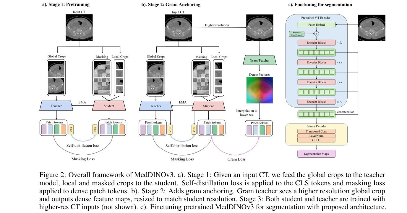
- MedDINOv3 adapts Meta’s DINOv3 vision transformer for CT and MRI segmentation using a simplified architecture and a three stage domain adaptive pretraining recipe on 3.87 million CT slices called CT-3M.
- It beats the strongest supervised CNN baseline, nnU-Net, on organ segmentation by 2.6 percentage points of Dice on AMOS22 and 5.49 points on BTCV, while roughly matching it on two tumor segmentation benchmarks.
- Four datasets used to build the CT-3M pretraining corpus, BTCV, LiTS, KiTS, and AMOS22, are the exact same four datasets used later to report the headline evaluation numbers.
- The paper’s own ablation shows the second of its three pretraining stages, gram anchoring, produced a small decrease rather than an improvement in this particular experiment.
- On the two tumor datasets, MedDINOv3 leads on the overlap based Dice metric but nnU-Net still wins or ties on the boundary sensitive normalized surface Dice metric, a distinction the results section does not fully spell out.
- Every benchmark number comes from a single fold of a five fold cross validation split rather than an averaged result, which the authors attribute to computational cost.
A note before you read further
This article explains a published engineering paper about an automated image segmentation method. It is not medical advice, it does not diagnose anything, and it is not a substitute for a radiologist, a radiation oncologist, or a qualified clinician reviewing an actual scan. Nothing described here has cleared regulatory review for clinical use, and readers with questions about organ imaging, tumor detection, or treatment planning should talk to a medical professional rather than a research paper.
The problem behind every contouring workflow
CT and MRI scans are the backbone of modern radiology, and outlining organs at risk and tumors inside those scans drives everything from surgical planning to radiotherapy dosing. Manual contouring is accurate but slow, and every specialized deep learning model built to automate it tends to work well only on the scanner, protocol, and patient population it was trained on. That narrowness is the generalization problem the field keeps circling back to, and it is the reason foundation models, trained once on enormous unlabeled datasets and then adapted to many downstream tasks, have become an appealing shortcut.
The catch, as the MedDINOv3 authors put it plainly in their introduction, is that billion scale medical imaging data does not exist the way billion scale internet photo data does, mostly because of patient privacy constraints. That leaves an open question. Can a model that learned to see using ordinary photographs of cats, cars, and street scenes actually transfer anything useful to a CT slice of a kidney. Their answer is a qualified yes, provided the model gets further pretraining on medical images before it ever sees a labeled segmentation mask.
Where earlier attempts at this stalled
Vision transformers have been tried in medical segmentation for years without fully displacing convolutional networks. TransUNet folded transformer layers into a U-Net bottleneck. UNETR went further and used a plain ViT as the entire encoder, which the authors describe as a shift toward transformer heavy designs. SwinUNETR followed with a hierarchical Swin transformer backbone. Despite all of that architectural effort, a widely cited nnU-Net benchmarking study found that the specialized convolutional nnU-Net pipeline remains a genuinely strong baseline that transformer based methods struggle to beat consistently.
On the pretraining side, DINOv2 already showed that self supervised vision transformers can learn strong general purpose features from natural images alone. A prior study by Baharoon and colleagues tested whether those DINOv2 features transfer to radiology and found they hold up reasonably well for classification but lag behind domain pretrained models for segmentation specifically. A separate line of work called Primus tried stripping transformer segmentation architectures down to their essentials, using only a lightweight transposed convolution decoder, and showed that a bare bones transformer can approach CNN performance in 3D volumetric segmentation. MedDINOv3 borrows heavily from Primus’s minimalist decoder philosophy while trying to fix two things Primus left on the table, weak spatial detail from using only the final transformer layer, and a patch size choice that the authors argue does not suit DINOv3 style pretraining.
How MedDINOv3 puts the pieces together
The architecture starts from a DINOv3 ViT-B encoder pretrained on 1.689 billion natural images, paired with the same style of lightweight decoder Primus uses, a short stack of transposed convolution, layer normalization, and GELU activation layers that upsample patch tokens back to a full resolution segmentation map. This design choice is deliberate. By keeping the decoder as thin as possible, the authors make sure any improvement in results can be credited to the transformer’s own representations rather than to a decoder doing most of the heavy lifting.
Revisiting plain vision transformers
The authors build up their architecture one refinement at a time and report each step’s effect on the AMOS22 abdominal organ dataset.
| Configuration | DSC percent | Change |
|---|---|---|
| Random init, Primus decoder, single scale, 640 resolution | 78.39 | baseline |
| DINOv3 pretrained init added | 81.35 | plus 2.96 |
| Multi scale token aggregation added | 83.45 | plus 2.10 |
| Resolution raised to 896 by 896 | 85.51 | plus 2.06 |
Two of these four steps matter most for understanding what actually makes the architecture work. Multi scale token aggregation addresses a real weakness of plain vision transformers, that a standard ViT segmentation head like Primus only reads the output of the very last transformer block, throwing away the finer grained spatial information that earlier blocks still carry. MedDINOv3 instead pulls patch tokens from four intermediate blocks, specifically blocks two, five, eight, and eleven, and concatenates them before the decoder sees them. The choice of exactly those four blocks is not itself ablated in the paper, so a reader cannot tell from this publication alone whether a different set of layers would do better or worse. The second big lever is simply training at higher resolution, 896 by 896 rather than 640 by 640, which the authors frame as a substitute for Primus’s approach of shrinking patch size from 16 to 8, an approach they argue is computationally heavier and poorly matched to how DINOv3 was originally pretrained.
Domain adaptive pretraining on CT-3M
With the architecture settled, the second half of the paper is about further pretraining that architecture on medical images before any labeled fine tuning happens. The authors curated CT-3M, a collection of 3,868,833 axial CT slices drawn from sixteen public datasets covering more than one hundred anatomical structures across the abdomen, thorax, and pelvis. They then run a three stage recipe adapted from DINOv3’s own training procedure.
Stage one is a direct DINOv2 style recipe, combining a global image level loss that enforces consistency between different crops of the same scan, a patch level loss that reconstructs masked local regions, and a regularization term that spreads features apart in the embedding space so they do not collapse onto each other.
Stage two adds gram anchoring, a mechanism meant to stop the quality of patch level features from eroding as training keeps optimizing for the coarser global objective. It works by comparing the Gram matrix, the full set of pairwise similarities between every patch in an image, produced by the current student model against the same matrix produced by an earlier snapshot of the model called the Gram teacher, and penalizing the student when the two drift apart. Stage three then simply continues training while mixing in higher resolution crops, so the model that eventually gets fine tuned for segmentation has already seen CT images at something closer to the resolution it will be evaluated on.
Key takeaway
Every refinement in this paper follows a consistent philosophy, keep the decoder minimal and push as much of the representational work as possible into the pretrained transformer, then spend engineering effort on giving that transformer better inputs, more scales of tokens, higher resolution, and CT specific pretraining, rather than on decoder complexity.
What the benchmark numbers actually show
MedDINOv3 is evaluated against three baselines, nnU-Net as the strongest supervised CNN, SegFormer as a natural image transformer segmentation model, and DINO U-Net, a newer architecture that also integrates DINOv3 but keeps its encoder backbone frozen during fine tuning rather than updating it.
| Method | AMOS22 DSC | KiTS23 DSC | LiTS DSC | BTCV DSC | KiTS23 NSD | LiTS NSD |
|---|---|---|---|---|---|---|
| nnU-Net | 84.81 | 69.15 | 75.00 | 73.30 | 64.85 | 53.02 |
| SegFormer | 78.50 | 57.73 | 65.45 | 37.04 | 47.65 | 35.98 |
| DINO U-Net, frozen encoder | 80.90 | 59.77 | 72.89 | 66.88 | 51.05 | 48.25 |
| MedDINOv3 | 87.38 | 70.68 | 75.28 | 78.79 | 62.67 | 53.01 |
On the two organ at risk datasets, AMOS22 and BTCV, the gains over nnU-Net are large and consistent across both Dice and boundary metrics, which is a genuinely strong result for a general purpose vision transformer going up against a highly tuned, task specific CNN pipeline. The story softens on the two tumor datasets. MedDINOv3 does edge out nnU-Net on raw Dice for both KiTS23 and LiTS, but Dice is fairly forgiving of small boundary errors when the overall region overlap is close. Look instead at normalized surface Dice, the metric built specifically to measure how well predicted boundaries track the true boundary, and nnU-Net actually wins on KiTS23 by more than two points and holds an effective tie on LiTS. Tumor boundaries in kidney and liver scans tend to be the hardest and most clinically consequential part of the segmentation task, since margin decisions in oncology often come down to exactly where a tumor edge sits, so this is not a minor asterisk.
The pretraining corpus quietly includes the test benchmarks
This is the detail most worth slowing down for. The paper lists sixteen source datasets that make up CT-3M, the collection used for self supervised domain adaptive pretraining, and that list explicitly includes BTCV, LiTS, KiTS, and AMOS22. Those are not similar datasets, they are the identical four datasets later used to report the paper’s headline segmentation benchmark results in Table 2. Self supervised pretraining does not use the segmentation labels, so this is not label leakage in the traditional sense, and it is a defensible design choice, since using diverse CT sources for domain adaptive pretraining is exactly what that stage is supposed to do. But it does mean the model has already seen the pixel level appearance, scanner characteristics, and patient population of every one of its four evaluation benchmarks before fine tuning even begins. A cleaner test of generalization would hold at least one evaluation dataset entirely out of the pretraining corpus, so a practitioner reading the reported gains as evidence of transfer to genuinely unseen institutions should treat that claim as unproven by this particular experiment, even though the architecture itself may well generalize fine.
A frozen encoder is not a fair fight
The other detail buried in the implementation section is that DINO U-Net, the closest competing method that also uses a DINOv3 backbone, is run with its encoder backbone frozen during fine tuning, following its own original paper’s setup, while MedDINOv3 fine tunes its encoder fully. Freezing a backbone is a legitimate design choice elsewhere, often used to save compute or preserve pretrained features, but it also caps how much a model can adapt to the target domain during fine tuning. Comparing a frozen backbone competitor against a fully fine tuned MedDINOv3 conflates two separate questions, whether MedDINOv3’s own architectural refinements and CT-3M pretraining are better, and whether full fine tuning simply beats a frozen backbone regardless of which pretrained weights sit underneath. The paper does not report a fully fine tuned DINO U-Net variant, so this specific comparison cannot fully isolate MedDINOv3’s contribution from that confound.
Gram anchoring did not clearly help here
The pretraining ablation table tells its own honest story. Stage one alone raises Dice from the 85.51 architectural baseline to 86.58. Adding stage two, gram anchoring, actually brings the score down slightly to 86.54, a decrease rather than an improvement, though a small one that likely sits within normal run to run noise. Stage three, high resolution adaptation, then pushes the score up to 87.38. The authors are candid about this in their own text, suggesting that gram anchoring exists mainly to prevent patch feature degradation that simply was not happening much during their stage one training, which they support with a qualitative visualization rather than a quantitative degradation metric. For a reader deciding whether to replicate all three pretraining stages in their own pipeline, the practical takeaway is that stage three, higher resolution adaptation, appears to be doing more work than the more complex gram anchoring machinery in stage two, at least in this specific setup.
Clinical translation gap
There is meaningful distance between winning on four public benchmarks and being ready for a real radiology or radiation oncology workflow. Every evaluation here uses a single fold of an 80 20 split rather than results averaged across the full five fold cross validation that AMOS22, KiTS23, LiTS, and BTCV were designed around, and the authors attribute this directly to computational cost. That means the reported numbers, gains of a few percentage points in Dice, do not come with confidence intervals or variance estimates, which makes it hard to know how much of the reported edge over nnU-Net would hold up on a different fold or a different random seed. Deployment in an actual clinical pipeline would also need to handle 3D volumetric consistency, since MedDINOv3 operates on 2D axial slices, and the paper does not report how slice level predictions are reconciled into a single coherent 3D organ or tumor volume, nor does it report inference throughput or how the approach would integrate with existing treatment planning software.
Key takeaway
The organ at risk results on AMOS22 and BTCV are the strongest and most consistent part of this paper, holding up on both overlap and boundary metrics. The tumor segmentation results are a genuine step forward on Dice but a wash or a slight loss on boundary accuracy against nnU-Net, and boundary accuracy is often the number that matters most for tumor margins in practice.
Clinical limitations
A few constraints deserve to be named directly for anyone considering this work in a clinical research context. The evaluation datasets, while genuinely diverse in anatomy, are all public research benchmarks rather than fresh multi center clinical data, and as noted above four of them were also part of the self supervised pretraining corpus, which narrows how confidently the results speak to performance on a hospital’s own unseen scanner and patient population. KiTS23 covers 489 CT volumes and LiTS covers 131, both modest by the standards of a clinical validation study, and organ prevalence and tumor morphology can vary meaningfully across sites in ways a single benchmark cannot capture. This is a preprint posted to arXiv, and while the code has been released publicly, the work has not yet gone through the kind of independent peer review a journal publication would require before its claims should be treated as settled.
Honest limitations of the paper itself
The authors are transparent about several of these points themselves, describing gram anchoring as providing only marginal benefit in their setting rather than overselling it, and noting plainly that results come from a single cross validation fold due to computational constraints. What they do not foreground as clearly is the overlap between CT-3M’s source datasets and the evaluation benchmarks, or the frozen versus fine tuned encoder asymmetry in the DINO U-Net comparison, both of which a careful reader needs to reconstruct from the implementation details rather than the results narrative. The paper also does not report model size, parameter count, training time, or inference speed for MedDINOv3 relative to nnU-Net, information that would matter a great deal to anyone weighing whether the accuracy gains are worth the added computational cost of a full vision transformer pipeline.
Where this fits going forward
MedDINOv3 lands a real point in the ongoing argument between specialized CNNs and adapted vision transformers for medical segmentation, showing that a genuinely simple architecture, a pretrained transformer encoder plus a thin decoder, can beat nnU-Net on organ segmentation once it gets the right combination of multi scale tokens, higher resolution training, and CT specific pretraining. That is a meaningful data point in a field where transformer based methods have repeatedly struggled to clear the CNN bar on dense prediction tasks.
The conceptual shift worth tracking is the idea that a general purpose vision foundation model trained on ordinary photographs can be steered into a specialized medical tool through pretraining alone, without redesigning the underlying transformer. If that pattern holds beyond CT, it suggests hospitals and research groups might increasingly share a common foundation model backbone across many imaging tasks rather than training a new specialized network for every organ and every modality, which would be a genuine efficiency gain for a field that currently reinvents its architecture for nearly every new segmentation problem.
The honest gaps that remain are the ones a careful next study would need to close. Evaluating on at least one CT dataset entirely excluded from CT-3M pretraining would give a cleaner read on true generalization. Running the full five fold cross validation with variance reporting would tell a reader how stable these gains actually are. And extending the boundary accuracy analysis beyond the tumor datasets, where the NSD story already complicates the Dice headline, would clarify whether the same pattern shows up elsewhere.
None of this diminishes the underlying engineering contribution. Getting a plain vision transformer to beat nnU-Net at all is a nontrivial result given how many prior attempts have fallen short, and the architectural ablation in Table 1 is a genuinely useful roadmap for anyone trying to replicate that success in their own pipeline. The value of reading past the abstract here is not to dismiss the work but to know precisely which parts of its story are load bearing and which parts are doing less than the framing suggests.
For a field that keeps chasing the promise of one foundation model serving many imaging tasks, MedDINOv3 is a useful and mostly honest waypoint, strong on organs, more complicated on tumor boundaries, and a reminder that a pretraining corpus overlapping the test set is a detail worth checking in every foundation model paper that reports a big generalization number.
Frequently asked questions
What problem is MedDINOv3 trying to solve. It adapts DINOv3, a vision foundation model originally trained on natural internet images, into a backbone for segmenting organs and tumors in CT and MRI scans, aiming for better generalization than task specific models.
Does MedDINOv3 actually beat nnU-Net. Yes on organ at risk segmentation across both Dice and boundary metrics on AMOS22 and BTCV. On tumor segmentation it wins on Dice for KiTS23 and LiTS but nnU-Net still wins or ties on the boundary sensitive normalized surface Dice metric for those same two datasets.
What is gram anchoring and did it help. It is the second of three pretraining stages, designed to stop patch level feature quality from degrading during self supervised training. In this paper’s own ablation it produced a very slight decrease in Dice rather than an improvement, which the authors attribute to patch quality not degrading much in their setup to begin with.
Is there a concern with how the model was tested. Yes. Four of the sixteen datasets used to build the CT-3M pretraining corpus, BTCV, LiTS, KiTS, and AMOS22, are the same four datasets later used as evaluation benchmarks, which means the model had already seen unlabeled images from those exact sources before fine tuning.
Is this ready for use in a hospital. No. It is a research preprint evaluated on a single cross validation fold with no reported inference speed or 3D volumetric reconciliation strategy, and it has not undergone clinical validation or regulatory review.
Where can I read the original paper or see the code. The full preprint and the authors’ public code release are linked in the citation box below.
Read the original preprint for the full architecture diagrams, complete results tables, and dataset details.
Read the paper on arXiv View the code on GitHubLi, Y., Wu, Y., Lai, Y., Hu, M., and Yang, X. MedDINOv3, How To Adapt Vision Foundation Models For Medical Image Segmentation. arXiv:2509.02379, posted September 2, 2025, revised October 15, 2025.
This analysis is based on the published paper and an independent evaluation of its claims.
Related reading
Complete PyTorch implementation
The following is a full, runnable reimplementation of MedDINOv3’s core ideas based on the equations and architectural description in the paper, including multi scale token aggregation from a ViT encoder, the lightweight transposed convolution decoder, the gram anchoring loss, a combined training loop covering the segmentation objective, an evaluation function reporting Dice, and a smoke test on random dummy data.
# meddinov3.py
# Reimplementation of MedDINOv3 (Li, Wu, Lai, Hu, Yang 2025) core modules
# Assumes a ViT style encoder is available (e.g. a DINOv3 or DINOv2 checkpoint).
# The encoder wrapper below is a lightweight stand in exposing intermediate
# patch tokens, since a real pretrained DINOv3 backbone is not bundled here.

import math
import torch
import torch.nn as nn
import torch.nn.functional as F


class PatchEmbed(nn.Module):
    def __init__(self, img_size=896, patch_size=16, in_chans=1, embed_dim=768):
        super().__init__()
        self.grid_size = img_size // patch_size
        self.num_patches = self.grid_size * self.grid_size
        self.proj = nn.Conv2d(in_chans, embed_dim, kernel_size=patch_size, stride=patch_size)

    def forward(self, x):
        x = self.proj(x)  # (B, C, H/P, W/P)
        b, c, h, w = x.shape
        x = x.flatten(2).transpose(1, 2)  # (B, N, C)
        return x, (h, w)


class TransformerBlock(nn.Module):
    def __init__(self, dim, num_heads=12, mlp_ratio=4.0, drop_path=0.0):
        super().__init__()
        self.norm1 = nn.LayerNorm(dim)
        self.attn = nn.MultiheadAttention(dim, num_heads, batch_first=True)
        self.norm2 = nn.LayerNorm(dim)
        hidden = int(dim * mlp_ratio)
        self.mlp = nn.Sequential(
            nn.Linear(dim, hidden), nn.GELU(), nn.Linear(hidden, dim)
        )
        self.drop_path = drop_path

    def forward(self, x):
        y = self.norm1(x)
        attn_out, _ = self.attn(y, y, y, need_weights=False)
        x = x + attn_out
        x = x + self.mlp(self.norm2(x))
        return x


class ViTEncoder(nn.Module):
    """Minimal ViT-B style encoder exposing intermediate block outputs,
    standing in for a pretrained DINOv3 backbone. Blocks are 1 indexed
    to match the paper's block 2, 5, 8, 11 selection."""
    def __init__(self, img_size=896, patch_size=16, in_chans=1, embed_dim=768, depth=12, num_heads=12):
        super().__init__()
        self.patch_embed = PatchEmbed(img_size, patch_size, in_chans, embed_dim)
        num_patches = self.patch_embed.num_patches
        self.pos_embed = nn.Parameter(torch.zeros(1, num_patches, embed_dim))
        nn.init.trunc_normal_(self.pos_embed, std=0.02)
        self.blocks = nn.ModuleList([TransformerBlock(embed_dim, num_heads) for _ in range(depth)])
        self.embed_dim = embed_dim

    def forward(self, x, return_layers=(2, 5, 8, 11)):
        tokens, grid = self.patch_embed(x)
        tokens = tokens + self.pos_embed
        collected = {}
        for i, blk in enumerate(self.blocks, start=1):
            tokens = blk(tokens)
            if i in return_layers:
                collected[i] = tokens
        return collected, grid


class MultiScaleTokenDecoder(nn.Module):
    """Aggregates tokens from four intermediate blocks and upsamples
    them back to full resolution using stacked transposed convolutions,
    mirroring the Primus style decoder used in MedDINOv3."""
    def __init__(self, embed_dim=768, num_layers=4, num_classes=1, patch_size=16):
        super().__init__()
        fused_dim = embed_dim * num_layers
        self.fuse = nn.Conv2d(fused_dim, embed_dim, kernel_size=1)
        num_up = int(math.log2(patch_size))  # e.g. patch_size 16 needs 4 doublings
        layers = []
        ch = embed_dim
        for _ in range(num_up):
            out_ch = max(ch // 2, num_classes)
            layers += [
                nn.ConvTranspose2d(ch, out_ch, kernel_size=2, stride=2),
                nn.LayerNorm([out_ch, 1, 1]) if False else nn.GroupNorm(1, out_ch),
                nn.GELU(),
            ]
            ch = out_ch
        self.up = nn.Sequential(*layers)
        self.head = nn.Conv2d(ch, num_classes, kernel_size=1)

    def forward(self, token_dict, grid, layer_ids, out_size):
        h, w = grid
        feats = []
        for lid in layer_ids:
            t = token_dict[lid]  # (B, N, C)
            b, n, c = t.shape
            t = t.transpose(1, 2).reshape(b, c, h, w)
            feats.append(t)
        fused = torch.cat(feats, dim=1)
        fused = self.fuse(fused)
        up = self.up(fused)
        logits = self.head(up)
        logits = F.interpolate(logits, size=out_size, mode="bilinear", align_corners=False)
        return logits


class MedDINOv3(nn.Module):
    def __init__(self, img_size=896, patch_size=16, in_chans=1, embed_dim=768,
                 depth=12, num_heads=12, num_classes=1, layer_ids=(2, 5, 8, 11)):
        super().__init__()
        self.encoder = ViTEncoder(img_size, patch_size, in_chans, embed_dim, depth, num_heads)
        self.decoder = MultiScaleTokenDecoder(embed_dim, len(layer_ids), num_classes, patch_size)
        self.layer_ids = layer_ids

    def forward(self, x):
        token_dict, grid = self.encoder(x, return_layers=self.layer_ids)
        logits = self.decoder(token_dict, grid, self.layer_ids, out_size=x.shape[-2:])
        return logits


def gram_anchoring_loss(student_tokens, gram_teacher_tokens):
    """L_Gram = || X_S X_S^T - X_G X_G^T ||_F^2, per paper equation 2.
    Both inputs are L2 normalized (B, N, C) patch token tensors."""
    xs = F.normalize(student_tokens, dim=-1)
    xg = F.normalize(gram_teacher_tokens, dim=-1)
    gram_s = torch.bmm(xs, xs.transpose(1, 2))
    gram_g = torch.bmm(xg, xg.transpose(1, 2))
    diff = gram_s - gram_g
    return (diff ** 2).sum(dim=(1, 2)).mean()


def dice_loss(pred, target, eps=1e-6):
    pred = torch.sigmoid(pred)
    num = 2 * (pred * target).sum(dim=(1, 2, 3)) + eps
    den = pred.sum(dim=(1, 2, 3)) + target.sum(dim=(1, 2, 3)) + eps
    return 1 - (num / den).mean()


def segmentation_loss(logits, target):
    return F.binary_cross_entropy_with_logits(logits, target) + dice_loss(logits, target)


def train_one_epoch(model, loader, optimizer, device):
    model.train()
    running = 0.0
    for images, masks in loader:
        images, masks = images.to(device), masks.to(device)
        optimizer.zero_grad()
        logits = model(images)
        loss = segmentation_loss(logits, masks)
        loss.backward()
        optimizer.step()
        running += loss.item() * images.size(0)
    return running / len(loader.dataset)


@torch.no_grad()
def evaluate(model, loader, device):
    model.eval()
    total_dice, n = 0.0, 0
    for images, masks in loader:
        images, masks = images.to(device), masks.to(device)
        logits = model(images)
        pred = (torch.sigmoid(logits) > 0.5).float()
        dice = (2 * (pred * masks).sum(dim=(1, 2, 3)) + 1e-6) / (
            pred.sum(dim=(1, 2, 3)) + masks.sum(dim=(1, 2, 3)) + 1e-6
        )
        total_dice += dice.sum().item()
        n += images.size(0)
    return {"mDice": total_dice / n}


if __name__ == "__main__":
    # smoke test on random dummy data, confirms shapes and gradient flow only
    # using a small image size and shallow depth to keep this fast to run
    device = torch.device("cuda" if torch.cuda.is_available() else "cpu")
    img_size, patch_size, embed_dim, depth = 128, 16, 64, 4
    layer_ids = (1, 2, 3, 4)

    model = MedDINOv3(
        img_size=img_size, patch_size=patch_size, in_chans=1,
        embed_dim=embed_dim, depth=depth, num_heads=4,
        num_classes=1, layer_ids=layer_ids,
    ).to(device)

    batch_size = 2
    dummy_images = torch.randn(batch_size, 1, img_size, img_size, device=device)
    dummy_masks = (torch.rand(batch_size, 1, img_size, img_size, device=device) > 0.7).float()

    optimizer = torch.optim.AdamW(model.parameters(), lr=1e-4)

    model.train()
    logits = model(dummy_images)
    loss = segmentation_loss(logits, dummy_masks)
    loss.backward()
    optimizer.step()
    print("training step ok, loss =", loss.item(), "logits shape =", tuple(logits.shape))

    # quick check that the gram anchoring loss runs on matching token shapes
    with_tokens, _ = model.encoder(dummy_images, return_layers=layer_ids)
    student_tokens = with_tokens[layer_ids[-1]]
    gram_teacher_tokens = student_tokens.detach() + 0.01 * torch.randn_like(student_tokens)
    g_loss = gram_anchoring_loss(student_tokens, gram_teacher_tokens)
    print("gram anchoring loss ok, value =", g_loss.item())

    model.eval()
    with torch.no_grad():
        eval_logits = model(dummy_images)
    assert eval_logits.shape == (batch_size, 1, img_size, img_size)
    print("eval step ok, logits shape =", tuple(eval_logits.shape))
    print("smoke test passed")
Pingback: SegTrans: The Breakthrough Framework That Makes AI Segmentation Models Vulnerable to Transfer Attacks - aitrendblend.com
Pingback: Revolutionizing Medical Imaging: How a Compact, Programmable Ultrasound Array Unlocks High-Contrast Elastography for Bones and Tumors - aitrendblend.com
I don’t think the title of your article matches the content lol. Just kidding, mainly because I had some doubts after reading the article.
Your point of view caught my eye and was very interesting. Thanks. I have a question for you.