
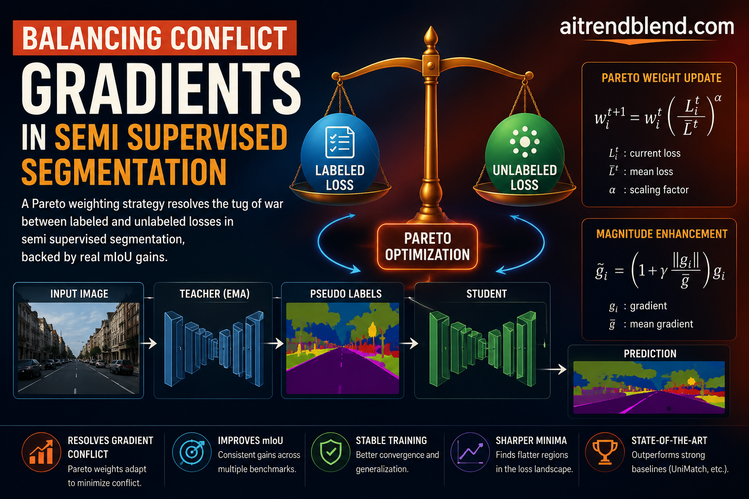
Key points
- Supervised and unsupervised gradients in semi supervised segmentation frequently point in conflicting directions, confirmed by negative cosine similarity measured across ten thousand training iterations on Pascal VOC.
- The paper proposes a Pareto Optimization Strategy, POS, that solves a small closed form problem each step to find blended weights that never work against either loss.
- POS on its own tends to favor the unsupervised gradient so strongly that it settles into a sharp minimum, which the authors show hurts generalization.
- A second step called the Magnitude Enhancement Operation rescales the blended gradient so the model lands in a flatter, more generalizable region instead.
- Dropped into UniMatch and UniMatch V2 with no other changes, the combined method lifts mIoU by roughly one to two and a half points across Pascal VOC, COCO, and Cityscapes, with the biggest gains in the most label scarce splits.
The problem nobody was measuring
Semantic segmentation needs pixel level labels, and pixel level labels are expensive. A single Cityscapes style image can take the better part of an hour to annotate carefully. Semi supervised segmentation exists to get around that cost by training on a small labeled set alongside a much larger unlabeled one, usually through a teacher student setup. The teacher, often an exponential moving average of the student, looks at a weakly augmented version of an unlabeled image and produces pseudo labels. The student then has to reproduce those same predictions on a strongly augmented version of the same image. Add a standard supervised loss on the labeled data, sum the two losses with equal weight, and you have most of the methods that have defined this field for the last few years, UniMatch among them.
That equal weighting choice is where this paper starts pulling threads. The authors call it the uniform strategy and point out that nobody ever really checked whether averaging two losses that were never designed to agree with each other is actually a sound thing to do. So they measured it. Across ten thousand iterations of training on Pascal under the widely used 366 partition protocol, they computed the cosine similarity between the gradient coming from the supervised loss and the gradient coming from the unsupervised loss at every step. If the two gradients agreed, the number would sit above zero. It did not, consistently. A meaningful fraction of training steps showed negative cosine similarity, meaning the two objectives were actively working against each other and the network was being nudged by two forces pulling in opposite directions at the same moment.
This matters because gradient descent with two conflicting sources of supervision is not the same problem as gradient descent with one. When the supervised and unsupervised gradients disagree, summing them with fixed weights does not average out the conflict, it just picks a direction that may satisfy neither loss particularly well. The paper frames this explicitly as a multi objective optimization problem, drawing on ideas from Pareto optimality that go back decades in operations research and that have more recently found their way into multi task learning through work like Sener and Koltun’s framing of multi task learning as multi objective optimization.
What came before
The related work section places this paper inside four active threads in semi supervised segmentation research. One line of work pushes on data augmentation, AugSeg and RandAugment among them, expanding the space of perturbations a student network has to stay consistent across. A second line optimizes the teacher itself, with methods like Switch addressing the coupling problems that come from a naive exponential moving average teacher through dual teacher ensembling. A third line brings in external knowledge, LOGIC through symbolic reasoning and SemiVL through CLIP based text priors, to improve the quality of pseudo labels before they ever reach the student. A fourth line pushes on consistency itself, RankMatch exploiting pixel correlations and MPMC folding in contextual class information. None of these four directions touch the actual arithmetic of how the two losses get combined once they exist. That gap is exactly where this paper positions itself, and it is a fair gap to claim, because a survey of the cited baselines shows every one of them either summing the two losses directly or applying a fixed scalar weight decided in advance.
How the Pareto Optimization Strategy works
The method itself is not a bigger network or a fancier augmentation pipeline. It changes exactly one thing, how the two gradients get combined at each training step, and it does that with a small piece of convex optimization rather than a hand tuned hyperparameter.
Let g_s be the gradient computed from the supervised loss on a mini batch and g_u be the gradient computed from the unsupervised loss on the same step. Instead of fixing the mixing weights at one half and one half, the paper solves for weights alpha_s and alpha_u that minimize the squared norm of the combined gradient, subject to both weights being non negative and summing to one.
This looks abstract until you notice what it is actually asking for. It is asking, out of every possible weighted blend of these two gradients, which blend has the smallest magnitude. That sounds backwards at first, why would you want a small gradient, until you remember a classical result from multi objective optimization. If the minimum norm solution to this problem is zero, the current parameters are Pareto stationary, meaning no small step can improve one loss without making the other worse, which is a necessary condition for having reached a jointly optimal point. If the minimum norm is not zero, the resulting blended gradient is guaranteed to be a descent direction for both losses simultaneously. Move along it and neither loss goes up. That guarantee simply does not exist for a fixed fifty fifty blend, which can easily point in a direction that helps one loss while actively hurting the other whenever the two gradients disagree.
The genuinely useful part is that this optimization problem has a closed form solution, so it costs almost nothing extra to compute at every step. Let beta be the angle between g_s and g_u. The solution falls into one of three cases depending on how that angle compares to the ratio of the two gradient norms.
In practice the middle case is the common one, where both gradients get a nonzero share and the exact ratio depends on their relative angle and magnitude at that particular step. Because the two losses are computed independently during training anyway, plugging these weights back into the total loss function costs nothing beyond the closed form calculation itself. That total loss, with the dynamic weights substituted in, is just L equal to alpha_s times the supervised loss plus alpha_u times the unsupervised loss, evaluated fresh at every iteration instead of fixed once at the start of training.
A surprising asymmetry, and why it appears
Once the authors had POS running, they went looking for a pattern in the weights it assigned. What they found was consistent across the whole training run, POS leans toward the unsupervised gradient far more often than not, typically assigning it more than half the weight.
The explanation traces back to a simpler observation about gradient magnitude. Figure 3 in the paper plots the distribution of gradient magnitudes from the two branches directly, and the numbers are stark. The mean magnitude of the unsupervised gradient sits at 0.529, while the supervised gradient averages 2.242, more than four times larger. The batch sampling covariance shows an even bigger gap, 0.110 for the unsupervised branch against 1.584 for the supervised one, a difference the authors note is consistently more than threefold in their experiments.
Why would labeled data produce a noisier, larger gradient than unlabeled data. The paper’s answer comes down to task difficulty. Training against ground truth labels is a genuinely hard optimization target, there is no slack, the model either matches the true class boundary or it does not. Training against pseudo labels from a teacher network is comparatively gentle, because the teacher is homologous to the student itself, an exponential moving average or a direct copy, so its predictions share the same biases and blind spots as the student. Matching a teacher that already thinks similarly to you is an easier objective than matching a hand drawn ground truth mask, and easier objectives tend to produce smaller, steadier gradients. That asymmetry is exactly why the closed form Pareto solution keeps tilting toward the unsupervised branch, the math is compensating for the fact that the supervised branch would otherwise dominate the combined direction on magnitude alone.
The paper is careful to connect this back to prior work rather than presenting it as a brand new discovery in isolation, noting that the tendency for labeled data to dominate training has also been observed in Allspark, a related paper on reborn labeled features. What is new here is quantifying exactly how that dominance shows up in gradient statistics and showing what a principled weighting scheme does in response to it.
The catch, sharp minima
Here is where the paper does something a lot of methods papers skip, it goes looking for the downside of its own proposed fix instead of stopping at the headline number.
The authors reframe stochastic gradient descent on mini batches as sampling from a noisy estimate of the true full batch gradient, following a standard framework from prior work on the anisotropic noise inherent to SGD. Under the uniform strategy, the noise injected at each step has a covariance proportional to the sum of the supervised and unsupervised sampling covariances, scaled by a constant factor tied to the fixed one half weighting. Swap in the POS weights, and because those weights are usually pushed toward the smaller magnitude, lower covariance unsupervised branch, the effective noise in the update shrinks.
Less training noise sounds like a good thing until you remember why SGD noise exists in the first place. That noise is part of what helps a network escape sharp, narrow minima and settle into flatter regions of the loss surface, which tend to generalize better to unseen data. The paper works through the algebra and shows that for a wide range of realistic covariance ratios between the two branches, POS on its own reduces the noise term enough to risk converging into a sharper minimum than the uniform strategy would, even though POS reaches a better training loss along the way. Table 4 backs this up empirically. Adding POS alone lifts Pascal mIoU from a 75.2 baseline to 77.0 at the ninety two split, a solid gain, but there is more headroom sitting on the table.
Magnitude Enhancement Operation, putting the noise back where it helps
The fix the authors land on is almost stubbornly simple given how much analysis led up to it. Rather than abandoning POS, they keep its conflict free direction and just rescale its magnitude to match what the uniform strategy would have produced.
Read left to right, the first fraction is just the POS direction normalized to a unit vector. The second term is the magnitude the plain uniform strategy would have used. Multiply them together and you get a gradient that points exactly where POS says to point, but travels as far as the uniform strategy would have traveled. The authors show that because POS tends to favor the smaller magnitude unsupervised gradient, this rescaling factor lambda works out to be greater than one, meaning the noise strength that POS had quietly suppressed gets restored.
Table 4 shows what that restoration buys. Adding the Magnitude Enhancement Operation on top of POS pushes Pascal mIoU from 77.0 to 77.6 at the ninety two split, and COCO climbs from 33.4 to 34.0 mIoU at the most extreme 1 over 512 label split. Figure 5 in the paper makes the mechanism visible directly, plotting the training loss landscape and the test performance landscape for all three strategies side by side. POS with MEO produces a visibly flatter, wider basin around its minimum in both plots, while the plain uniform strategy shows a narrower, more peaked region that the authors read as a sign of overfitting risk.
Testing it across architectures and datasets
The experiments avoid a common trap in this kind of paper, testing a clever idea on exactly one backbone and one dataset. POS and MEO get dropped into two different frameworks, the original UniMatch with a ResNet-101 backbone and DeepLabv3+ decoder, and the newer UniMatch V2 built on a DINOv2-S vision transformer backbone with a simple DPT decoder. Both variants are evaluated with no other changes to augmentation, learning rate schedule, or training length, which is exactly what you want to see if a claim is really about the loss weighting and not about some other tuning that snuck in alongside it.
Pascal VOC 2012
Pascal remains the classic benchmark here, twenty object classes across 1464 training and 1449 validation images. The gains are largest in the most label starved split.
| Backbone | 1/16 (92) | 1/8 (183) | 1/4 (366) | 1/2 (732) | Full (1464) |
|---|---|---|---|---|---|
| ResNet-101, UniMatch V1 | 75.2 | 77.2 | 78.8 | 79.9 | 81.2 |
| ResNet-101, UniMatch V1 + POS/MEO | 77.6 | 78.7 | 79.7 | 80.9 | 81.9 |
| DINOv2-S, UniMatch V2 | 79.0 | 85.5 | 85.9 | 86.7 | 87.8 |
| DINOv2-S, UniMatch V2 + POS/MEO | 80.7 | 86.8 | 87.2 | 87.5 | 88.3 |
At the ninety two image split, the most extreme test of how well a method uses scarce labels, the ResNet backbone gains 2.4 mIoU points and the transformer backbone gains 1.7. Both are meaningful jumps in a field where recent papers have often been fighting over fractions of a point.
COCO
COCO is the harder test, 118 thousand training images spread across 81 categories, evaluated under partition protocols as tight as one labeled image for every 512 unlabeled ones.
| Backbone | 1/512 | 1/256 | 1/128 | 1/64 | 1/32 |
|---|---|---|---|---|---|
| XC-65, UniMatch V1 | 31.9 | 38.9 | 44.4 | 48.2 | 49.8 |
| XC-65, UniMatch V1 + POS/MEO | 34.0 | 40.3 | 45.9 | 49.3 | 50.7 |
| DINOv2-S, UniMatch V2 | 39.3 | 45.4 | 53.2 | 55.0 | 57.0 |
| DINOv2-S, UniMatch V2 + POS/MEO | 40.9 | 46.8 | 54.3 | 56.2 | 57.7 |
The 1 over 512 split, where labeled data is scarcest relative to the size of the dataset, again shows the largest jump, 2.1 points on the CNN backbone and 1.6 on the transformer backbone.
Cityscapes
Cityscapes tests something different again, a smaller but denser dataset of urban driving scenes, 2975 training and 500 validation images across 19 remapped classes, at higher resolution crops than either of the other two datasets.
| Backbone | 1/16 (186) | 1/8 (372) | 1/4 (744) | 1/2 (1488) |
|---|---|---|---|---|
| ResNet-101, UniMatch V1 | 76.6 | 77.9 | 79.2 | 79.5 |
| ResNet-101, UniMatch V1 + POS/MEO | 77.6 | 78.5 | 79.8 | 80.4 |
| DINOv2-S, UniMatch V2 | 80.6 | 81.9 | 82.4 | 82.6 |
| DINOv2-S, UniMatch V2 + POS/MEO | 81.4 | 82.7 | 83.0 | 83.2 |
The gains here are more modest, roughly one point at the tightest split, which makes sense given how competitive the Cityscapes leaderboard already is among the cited baselines like BeyondPixels and CorrMatch. Still, the improvement holds in the same direction across every split and every backbone, which is the pattern you want to see from a change that is supposed to be a general fix rather than a lucky tuning result on one dataset.
What this means beyond one paper
The mechanism here is not tied to segmentation specifically. Any teacher student setup that sums a supervised loss and a consistency loss, which describes a large share of semi supervised learning broadly and not just the pixel dense version of it, is exposed to the same conflict this paper measured. The closed form Pareto weighting and the magnitude rescaling step are both generic enough to plug into other consistency based pipelines without much modification, and the paper’s own ablations across two very different backbone families, a convolutional ResNet and a vision transformer pretrained through DINOv2, suggest the fix is not exploiting some quirk of one particular architecture.
There is also a broader methodological lesson worth pulling out. It is easy to treat loss weighting as a minor implementation detail that gets a paragraph in the appendix. This paper treats it as the central object of study, measures it directly with cosine similarity plots instead of asserting a problem exists, and then goes one step further to interrogate its own proposed fix for a hidden cost before declaring victory. That kind of self skepticism, checking whether solving one problem quietly introduces another, is rarer in this literature than it should be.
Honest limitations
A few caveats are worth sitting with rather than glossing over. The sharp minima analysis in Section 3.3 relies on treating the supervised and unsupervised gradients as statistically independent random variables with fixed covariance structure, a simplifying assumption that lets the math stay tractable but is an approximation of what is actually a highly non stationary, correlated training process in practice. The magnitude rescaling in MEO uses the uniform strategy’s gradient norm as its reference point, which is a reasonable and empirically validated choice but is still a design decision rather than something derived purely from first principles, a different reference norm might behave differently and the paper does not sweep that choice.
The gains, while consistent, are also incremental rather than transformative, typically one to two and a half mIoU points on top of already strong baselines, and the Cityscapes results in particular show the smallest margins of the three datasets tested. Readers should also note this is a single paper’s results on standard academic benchmarks, all built on curated, relatively clean imagery, and the gradient magnitude statistics in Figure 3 were measured under one specific training setup on Pascal, so the exact numeric asymmetry between supervised and unsupervised gradient magnitudes should be read as illustrative of the phenomenon rather than as a universal constant that will reproduce identically on every dataset or architecture.
A working PyTorch implementation
The block below is a self contained, runnable implementation of the core mechanics described above, the closed form Pareto weight solver from Equation 6, the Magnitude Enhancement Operation from Equation 13, a minimal teacher student segmentation loop, and a smoke test on random dummy data so you can confirm it runs before pointing it at a real dataset.
# pareto_segmentation.py
# A minimal, runnable implementation of POS and MEO
# for balancing supervised and unsupervised gradients
# in a teacher student semi supervised segmentation setup.

import torch
import torch.nn as nn
import torch.nn.functional as F
import copy


def flatten_grads(params):
    # Concatenate all parameter gradients into a single 1D tensor.
    flat = []
    for p in params:
        if p.grad is not None:
            flat.append(p.grad.detach().reshape(-1))
    return torch.cat(flat)


def solve_pareto_weights(g_s, g_u, eps=1e-8):
    """
    Closed form solution to Equation 6 in the paper.
    g_s, g_u are flat 1D gradient tensors from the supervised
    and unsupervised losses respectively.
    Returns (alpha_s, alpha_u) with alpha_s + alpha_u == 1.
    """
    norm_s = torch.norm(g_s) + eps
    norm_u = torch.norm(g_u) + eps
    cos_beta = torch.dot(g_s, g_u) / (norm_s * norm_u)

    if cos_beta >= (norm_u / norm_s):
        return 0.0, 1.0
    if cos_beta >= (norm_s / norm_u):
        return 1.0, 0.0

    diff = g_s - g_u
    denom = torch.dot(diff, diff) + eps
    alpha_u = torch.dot(diff, g_s) / denom
    alpha_u = torch.clamp(alpha_u, 0.0, 1.0).item()
    alpha_s = 1.0 - alpha_u
    return alpha_s, alpha_u


def magnitude_enhancement(g_s, g_u, alpha_s, alpha_u, eps=1e-8):
    """
    Equation 13. Keeps the POS direction, rescales it to the
    magnitude the plain uniform (0.5, 0.5) blend would have had.
    """
    pos_grad = alpha_s * g_s + alpha_u * g_u
    pos_norm = torch.norm(pos_grad) + eps
    uniform_grad = 0.5 * g_s + 0.5 * g_u
    uniform_norm = torch.norm(uniform_grad)
    return (pos_grad / pos_norm) * uniform_norm


class TinySegNet(nn.Module):
    """A deliberately small encoder decoder for the smoke test."""

    def __init__(self, num_classes=4):
        super().__init__()
        self.enc = nn.Sequential(
            nn.Conv2d(3, 16, 3, padding=1), nn.ReLU(),
            nn.Conv2d(16, 32, 3, padding=1), nn.ReLU(),
        )
        self.head = nn.Conv2d(32, num_classes, 1)

    def forward(self, x):
        return self.head(self.enc(x))


def weak_aug(x):
    return x + 0.01 * torch.randn_like(x)


def strong_aug(x):
    return x + 0.15 * torch.randn_like(x)


def update_teacher(teacher, student, momentum=0.99):
    with torch.no_grad():
        for t_p, s_p in zip(teacher.parameters(), student.parameters()):
            t_p.data.mul_(momentum).add_(s_p.data, alpha=1 - momentum)


def train_step(student, teacher, opt, labeled_batch, unlabeled_batch,
               confidence_threshold=0.7, use_meo=True):
    x_l, y_l = labeled_batch
    x_u = unlabeled_batch

    student_params = [p for p in student.parameters() if p.requires_grad]

    # Supervised gradient, Equation 1
    opt.zero_grad()
    logits_l = student(x_l)
    loss_sup = F.cross_entropy(logits_l, y_l)
    loss_sup.backward()
    g_s = flatten_grads(student_params)

    # Pseudo labels from the teacher, Equation 2
    with torch.no_grad():
        teacher_logits = teacher(weak_aug(x_u))
        probs = F.softmax(teacher_logits, dim=1)
        confidence, pseudo_labels = probs.max(dim=1)
        valid_mask = confidence > confidence_threshold

    # Unsupervised gradient, Equation 3
    opt.zero_grad()
    student_logits = student(strong_aug(x_u))
    per_pixel_loss = F.cross_entropy(student_logits, pseudo_labels, reduction='none')
    if valid_mask.any():
        loss_unsup = (per_pixel_loss * valid_mask).sum() / valid_mask.sum().clamp(min=1)
    else:
        loss_unsup = per_pixel_loss.mean() * 0.0
    loss_unsup.backward()
    g_u = flatten_grads(student_params)

    # Solve for conflict free weights, Equation 6
    alpha_s, alpha_u = solve_pareto_weights(g_s, g_u)

    if use_meo:
        combined_flat = magnitude_enhancement(g_s, g_u, alpha_s, alpha_u)
    else:
        combined_flat = alpha_s * g_s + alpha_u * g_u

    # Write the combined gradient back into .grad and step once
    opt.zero_grad()
    pointer = 0
    for p in student_params:
        numel = p.numel()
        p.grad = combined_flat[pointer:pointer + numel].view_as(p).clone()
        pointer += numel
    opt.step()

    update_teacher(teacher, student)

    return {
        'loss_sup': loss_sup.item(),
        'loss_unsup': loss_unsup.item(),
        'alpha_s': alpha_s,
        'alpha_u': alpha_u,
    }


def evaluate(model, x, y, num_classes=4):
    model.eval()
    with torch.no_grad():
        preds = model(x).argmax(dim=1)
    ious = []
    for c in range(num_classes):
        pred_c = preds == c
        gt_c = y == c
        intersection = (pred_c & gt_c).sum().item()
        union = (pred_c | gt_c).sum().item()
        if union > 0:
            ious.append(intersection / union)
    model.train()
    return sum(ious) / max(len(ious), 1)


if __name__ == '__main__':
    torch.manual_seed(0)
    num_classes = 4

    student = TinySegNet(num_classes)
    teacher = copy.deepcopy(student)
    for p in teacher.parameters():
        p.requires_grad_(False)

    opt = torch.optim.SGD(student.parameters(), lr=0.01, momentum=0.9)

    # Dummy data smoke test, replace with real dataloaders
    x_labeled = torch.randn(2, 3, 32, 32)
    y_labeled = torch.randint(0, num_classes, (2, 32, 32))
    x_unlabeled = torch.randn(4, 3, 32, 32)

    x_val = torch.randn(2, 3, 32, 32)
    y_val = torch.randint(0, num_classes, (2, 32, 32))

    print('step  loss_sup  loss_unsup  alpha_s  alpha_u')
    for step in range(20):
        stats = train_step(
            student, teacher, opt,
            (x_labeled, y_labeled), x_unlabeled,
            confidence_threshold=0.0,
            use_meo=True,
        )
        if step % 5 == 0:
            print(f'{step:<5} {stats["loss_sup"]:<9.4f} {stats["loss_unsup"]:<11.4f} '
                  f'{stats["alpha_s"]:<8.3f} {stats["alpha_u"]:<8.3f}')

    val_iou = evaluate(student, x_val, y_val, num_classes)
    print(f'dummy validation mean IoU after smoke test: {val_iou:.4f}')
Conclusion
The core achievement of this paper is not a new architecture or a new augmentation trick, it is proof that a problem hiding in plain sight, how two unrelated losses get summed together, was quietly costing every method that skipped over it. By measuring gradient conflict directly instead of assuming it away, the authors turn a vague intuition that supervised and unsupervised signals might disagree into a concrete, closed form correction that any teacher student pipeline can adopt with minimal code changes.
The conceptual shift worth remembering is the move from static to dynamic weighting. Every prior method treated the balance between the two losses as a hyperparameter to be searched once and frozen. This paper treats it as a per step optimization problem that has an exact answer, derived from convex analysis rather than guessed at through a validation sweep. That reframing is what opens the door to the second contribution, because once you can compute the conflict free direction cheaply at every step, you can also inspect what that direction is doing to your training dynamics, which is exactly how the sharp minima problem got discovered in the first place.
Nothing about the gradient conflict argument is specific to pixel level segmentation. Any consistency based semi supervised method, image classification, object detection, even some multi task learning setups where a shared backbone serves two objectives with different noise characteristics, faces the same tension between a low variance signal and a high variance one. The Pareto weighting and magnitude rescaling recipe here is general enough that researchers working in adjacent areas could lift it with only modest adaptation.
The honest remaining gap is that this is still an empirical fix layered on top of a simplifying statistical model of training. The independence assumption between the two gradients, the choice to use the uniform strategy’s norm as the rescaling reference, and the reliance on standard academic benchmarks all leave room for follow up work to either tighten the theory or stress test the method on messier, real world data where labels are noisier and class distributions are far less balanced than Pascal or COCO.
Still, going from a one paragraph observation, that two losses might not agree, to a fully worked out solution with a proof of a hidden cost and a fix for that cost, inside one paper, is not a small piece of work. The next time a training run is not improving the way the loss curve suggests it should, this paper is a good reminder to ask whether the losses being summed together actually agree on where the model should go next.
Frequently asked questions
What is gradient conflict in semi supervised learning
Gradient conflict happens when the gradient computed from one training objective points in a different direction than the gradient from another objective, so that a step which improves one loss can make the other loss worse. In this paper the two objectives are a supervised loss on labeled data and an unsupervised consistency loss on unlabeled data, and the authors measured negative cosine similarity between the two gradients throughout training on Pascal VOC.
What does the Pareto Optimization Strategy actually change during training
It changes how the supervised and unsupervised gradients get combined at every step. Instead of a fixed fifty fifty split, it solves a small convex problem each iteration to find the blend with the smallest combined magnitude, which is mathematically guaranteed to be a descent direction for both losses at once whenever a conflict exists.
Why does POS favor the unsupervised gradient
Because the supervised gradient tends to have a much larger magnitude and a larger batch sampling covariance, roughly four times larger on average in the paper’s measurements. The closed form solution compensates for that imbalance by assigning more weight to the smaller, steadier unsupervised gradient.
What problem does the Magnitude Enhancement Operation solve
POS alone reduces the natural training noise that comes from mini batch sampling, which can push the model toward a sharp, narrow minimum that generalizes less well. The Magnitude Enhancement Operation keeps the conflict free direction from POS but rescales it back up to the magnitude the plain uniform strategy would have used, restoring enough noise to help the model settle into a flatter, more generalizable minimum.
How much does this improve segmentation accuracy in practice
Across Pascal VOC, COCO, and Cityscapes, combining POS and MEO with UniMatch and UniMatch V2 improved mIoU by roughly one to two and a half points depending on the dataset and the label split, with the largest gains showing up in the most label scarce settings such as the ninety two image Pascal split.
Does this method require a different network architecture
No. The paper tests it on both a convolutional ResNet-101 backbone with a DeepLabv3+ decoder and a DINOv2-S vision transformer backbone with a DPT decoder, and it improves results on both without any architectural changes, since the method only touches how the two loss gradients are combined during optimization.
Read the full paper for the complete derivations and additional ablations.
Read the paper (CVF Open Access) UniMatch code baseThe paper’s source PDF, hosted on the CVF Open Access repository, contains the full proofs behind Equations 6 through 12 along with additional loss landscape figures not covered in full detail above.
This analysis is based on the published paper and an independent evaluation of its claims.
Thanks for sharing. I read many of your blog posts, cool, your blog is very good. https://accounts.binance.info/ru/register?ref=O9XES6KU
Can you be more specific about the content of your article? After reading it, I still have some doubts. Hope you can help me. https://accounts.binance.info/ph/register?ref=IU36GZC4
Thank you for your sharing. I am worried that I lack creative ideas. It is your article that makes me full of hope. Thank you. But, I have a question, can you help me? https://accounts.binance.com/id/register?ref=UM6SMJM3