
Key points
- SSD-KD trains a compact MobileNetV2 student to mimic a much larger ResNet50 teacher using three kinds of knowledge at once, the teacher’s softened predictions, how the teacher relates different images to each other, and a new idea, how the teacher relates different feature channels within one single image.
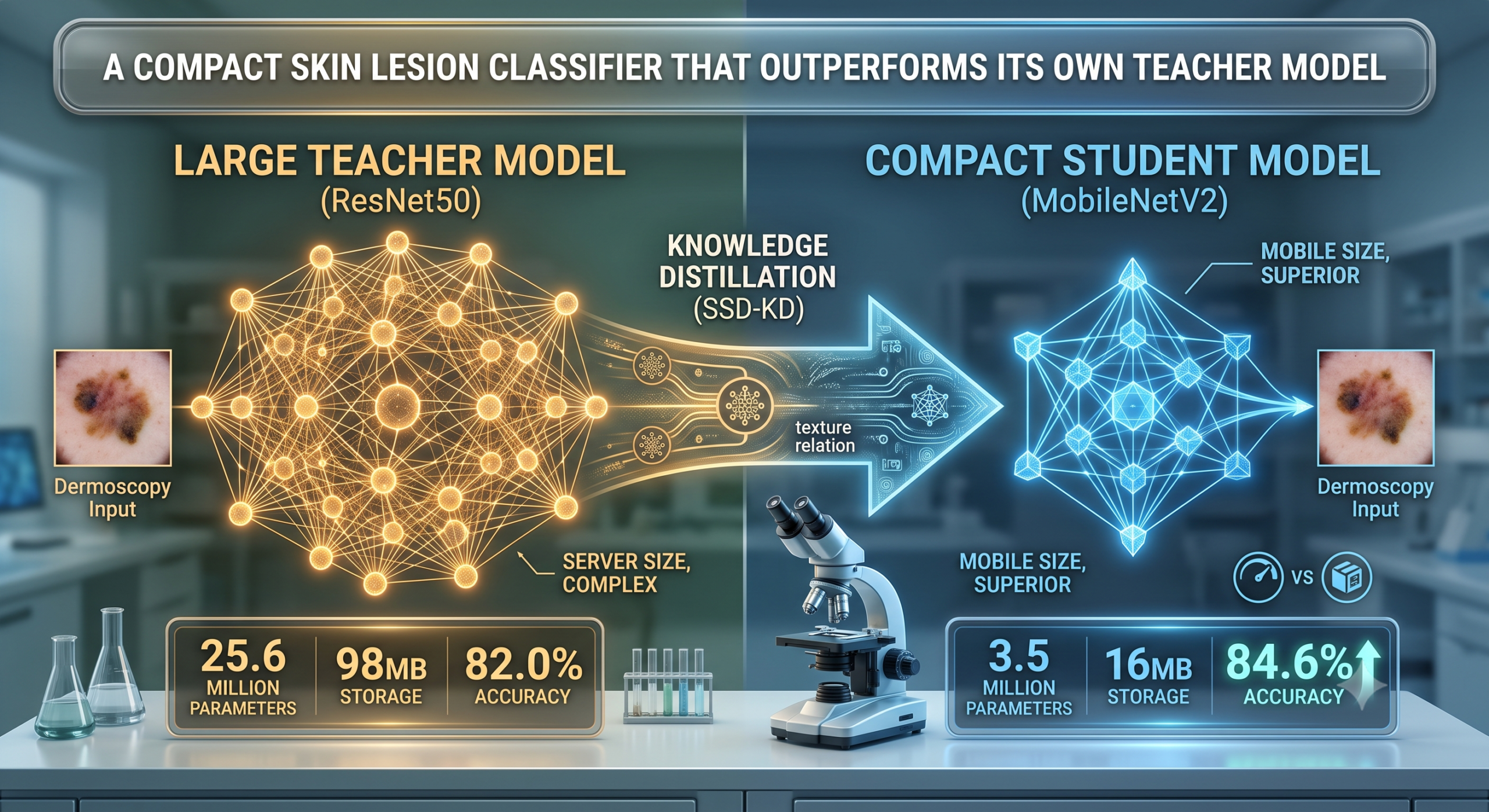
- On ISIC 2019, an eight class dermoscopy benchmark, the distilled MobileNetV2 reached 84.6 percent accuracy, actually surpassing its own 82.0 percent accurate teacher, while using about a seventh of the parameters and roughly half the inference time per step.
- The full method does not win every single metric in the paper’s own tables. Two simpler variants, one relying only on self supervision plus distance based relations, the other adding the new channel relation without self supervision, each posted a slightly higher AUC than the full SSD-KD method in at least one experiment.
- A leaderboard comparison the authors mention is worth reading carefully, since it compares against a non live version of the ISIC 2019 leaderboard on an eight class task rather than the official nine class challenge that includes an unknown lesion category.
- The biggest practical win may not be raw accuracy at all. The method cut the spread in per class precision scores across the eight, very unevenly sized disease categories by roughly half, which matters a lot for the rarest classes in the dataset.
The tradeoff this paper is trying to avoid
Skin cancer detection has become one of the clearer success stories for deep learning in medicine, with models trained on large dermoscopy image collections repeatedly matching or approaching dermatologist level accuracy on benchmark datasets. The catch is that the models winning these benchmarks tend to be large. ResNet50, a widely used architecture in this space, carries about 25.6 million parameters, needs 98 megabytes of storage, and runs at roughly 4.11 GFlops per image. That is a reasonable cost for a hospital server, but it is a real burden for a phone, a basic clinic laptop, or any embedded device without a dedicated graphics card, which is exactly the kind of hardware a screening tool would need to run on in a lower resource setting or a rural clinic.
The obvious fix is to use a smaller architecture built for exactly this constraint, something like MobileNetV2, which needs only about 3.5 million parameters and 16 megabytes. The problem is that smaller models trained the normal way, just on labeled images and a standard loss function, tend to underperform their larger counterparts by a real margin. In this paper’s own baseline comparison, a MobileNetV2 trained from scratch on the same data reached 75.4 percent accuracy against ResNet50’s 82.0 percent, a six and a half point gap that would matter quite a bit in a clinical screening context.
Knowledge distillation is the standard answer to this tradeoff, training the small student model to mimic a large pretrained teacher rather than just learning from labels alone. The idea traces back to Geoffrey Hinton and colleagues in 2015, and the basic recipe, softening a teacher’s output probabilities and training the student to match them alongside the true labels, has been extended in dozens of directions since. This paper’s contribution is specific. Most existing distillation methods applied to skin lesion diagnosis have stuck to comparing subject level category information, essentially just the teacher’s final answer, or at most how the teacher relates different training images to each other. The authors argue that ignores a real source of information sitting inside each individual image, the way different feature channels relate to each other within one lesion, which they connect to something dermatologists actually rely on, texture.
Three kinds of knowledge, stacked together
SSD-KD is built by layering three distinct distillation signals on top of each other, plus a self supervised training strategy borrowed and adapted from prior work, all combined into one loss function.
Logit based knowledge, the classic starting point
The first and oldest piece, referred to in the paper as BLKD, is the original Hinton style approach. The teacher’s output logits are softened with a temperature parameter, set to 5 here, turning a confident, near one hot prediction into a smoother probability distribution that reveals which wrong classes the teacher considers plausible. A Kullback-Leibler divergence loss pulls the student’s softened distribution toward the teacher’s. The authors make one meaningful change to the standard recipe here. Because ISIC 2019 is badly imbalanced, ranging from 12,875 images of melanocytic nevus down to just 239 images of dermatofibroma, they swap the usual cross entropy term for a weighted version, where each class is weighted by the inverse of how often it appears in training, giving the rare classes proportionally more influence on the gradient.
Inter instance relational knowledge, comparing images to each other
The second signal, called DRKD and borrowed from a 2019 paper by Park and colleagues, looks at how the teacher positions different images relative to each other in its learned embedding space, rather than just each image’s individual answer. Within a batch of training images, the teacher computes a distance between every pair of image embeddings and an angle between every triplet of embeddings, and the student is trained to reproduce those same relative distances and angles even if its own embedding space is a different shape entirely. The intuition is that a teacher’s sense of which lesions look similar to which other lesions carries information a single image’s logits cannot.
Intra instance relational knowledge, the paper’s actual contribution
The genuinely new piece is called CRKD, channel relational knowledge distillation, and it operates entirely within a single image rather than across a batch. At the last convolutional layer, a model produces many separate channel feature maps for one image, each one, in a rough sense, responding to a different visual pattern. CRKD computes the cosine similarity between every pair of those channel feature maps for a given image, producing a matrix that describes how those internal visual patterns relate to each other, then trains the student to reproduce the teacher’s version of that same matrix. Because a student model typically has fewer channels than its teacher, a small one by one convolution first projects the student’s channels up to match the teacher’s channel count before the comparison happens.
The authors frame this as a proxy for texture, since the relationships between different channel responses within one lesion image plausibly capture something about surface pattern and structure, a cue dermatologists already rely on directly when they look at a lesion under magnification. It is a reasonable interpretation, though it is worth being clear that it is exactly that, an interpretation of what a mathematical similarity matrix over feature channels is doing, rather than something independently verified against what a dermatologist would call texture.
Self supervision, adapted from a computer vision technique called SSKD
On top of these three, the authors borrow a self supervised training trick called SSKD from a 2020 computer vision paper by Xu and colleagues. Each image in a batch gets a randomly transformed version of itself, and both the teacher and student append a small extra prediction head that tries to solve a contrastive task, matching each transformed image back to its original among all the other images in the batch. The teacher’s contrastive similarity matrix becomes another target for the student to match through a KL divergence term. The stated motivation is that this contrastive task forces richer, more structured representations out of both models, and the authors cite separate evidence that self supervised training in general tends to help with class imbalance specifically, which lines up with their own imbalanced dataset.
Put together, the final SSD-KD loss combines the self supervised SSKD term, which already has the logit matching baked into it, with the inter instance DRKD term and the new intra instance CRKD term, each weighted by its own hyperparameter tuned through a staged grid search on a held out validation set.
The dataset and how the experiment was set up
All experiments run on ISIC 2019, a public dermoscopy benchmark containing 25,331 images across eight skin disease categories, malignant melanoma with 4,522 images, melanocytic nevus with 12,875, basal cell carcinoma with 3,323, actinic keratosis with 867, benign keratosis with 2,624, dermatofibroma with just 239, vascular lesion with 253, and squamous cell carcinoma with 628. That range, from under 250 images for the two rarest classes up to nearly 13,000 for the most common one, is a genuinely severe imbalance, over fifty to one between the largest and smallest categories, and it shapes several of the paper’s design choices.
Ten percent of the data was held out as a test set, with the remainder split 8 to 2 between training and validation. Images were resized to 224 by 224 pixels with standard augmentation, flips, brightness, contrast, and saturation adjustments, scaling, and added noise. Both the teacher and student started from ImageNet pretrained weights, then were fine tuned for 150 epochs using SGD with an initial learning rate of 0.001, momentum of 0.9, and weight decay of 0.001, with a batch size of 128 on a single NVIDIA Tesla V100. Evaluation used four metrics, accuracy, balanced accuracy, mean average precision, and area under the curve, the last two reported with their standard deviation across the eight classes specifically as a way to track how consistently the model performs on the rare categories, not just the common ones.
What the results actually show, including where the full method does not win
On the ResNet50 teacher paired with a MobileNetV2 student, the headline result holds up. SSD-KD reached 84.6 percent accuracy and 84.3 percent balanced accuracy, both higher than the 82.0 percent and 82.2 percent posted by the much larger ResNet50 teacher trained without any distillation involved at all. Compared against a plain MobileNetV2 trained without distillation, that is roughly a nine point accuracy gain from a model that did not grow by a single parameter.
| Configuration | Accuracy | Balanced accuracy | AUC | Mean average precision |
|---|---|---|---|---|
| ResNet50 teacher, no distillation | 82.0% | 82.2% | 0.975 ± 0.019 | 0.740 ± 0.108 |
| MobileNetV2 student, no distillation | 75.4% | 76.7% | 0.959 ± 0.035 | 0.625 ± 0.158 |
| MobileNetV2 with BLKD only | 83.8% | 82.4% | 0.976 ± 0.017 | 0.751 ± 0.103 |
| MobileNetV2 with SSKD only | 84.0% | 84.0% | 0.978 ± 0.017 | 0.759 ± 0.109 |
| MobileNetV2 with SSD-KD, full method | 84.6% | 84.3% | 0.977 ± 0.017 | 0.796 ± 0.081 |
Look closely at that AUC column. SSKD on its own, without the new channel relation piece at all, actually posted a marginally higher AUC, 0.978 against the full method’s 0.977. It is a small difference, well within what the standard deviations suggest could be noise, but it means the full SSD-KD method is not a strict, metric by metric improvement over every simpler alternative tested, it is the best choice on three of four headline metrics with mean average precision showing by far the largest and most meaningful gap. The same pattern shows up again on the paper’s second teacher and student pair.
A second architecture pair tells a similar but not identical story
To check whether the result generalizes beyond one specific architecture choice, the authors repeated the entire comparison with EfficientNetB7 as the teacher, 66.7 million parameters and 256 megabytes, and EfficientNetB0 as the student, 5.3 million parameters and 29 megabytes. The pattern holds, SSD-KD reached 86.6 percent accuracy and 85.8 percent balanced accuracy against the teacher’s 84.3 percent and 83.4 percent, again a student beating its own teacher. But the ablation table for this pair shows something worth flagging directly, an SSKD plus CRKD combination without the inter instance DRKD term posted an AUC of 0.980, noticeably higher than the full method’s 0.976. That is not a rounding difference, it is the single highest AUC anywhere in either ablation table, and it belongs to a simpler variant of the method rather than the full one.
The part of the story that matters most for an imbalanced dataset
Accuracy and AUC are useful headline numbers, but on a dataset where the rarest class has 239 images and the most common has almost 13,000, the standard deviation of mean average precision across the eight classes is arguably the more clinically relevant number, since it tracks how consistently a model performs across common and rare disease categories rather than averaging that variation away. Here the improvement is real and substantial. The plain MobileNetV2 without distillation had a mean average precision standard deviation of 0.158 across the eight classes, meaning wildly inconsistent performance between well represented and poorly represented diseases. SSD-KD brought that down to 0.081, roughly half. That is a genuinely strong result for an imbalanced medical dataset, arguably a stronger and more clinically meaningful claim than the headline accuracy number, and it is the kind of detail that a summary focused only on the top line accuracy would miss entirely.
What the activation maps suggest, with appropriate caution
To get some visual intuition for what distillation changed, the authors used Grad-CAM to generate class activation maps, comparing where the teacher model focuses its attention, where the undistilled student focuses, and where the distilled student focuses, across a handful of example images that also happened to include common dermoscopy artifacts, hair, ink markers, gel bubbles, and rulers. They report that the distilled student’s attention maps aligned more closely with the teacher’s than the undistilled student’s did, and that this alignment tracked with the student circumventing some of the artifact related errors it made without distillation, including a specific example of 17 melanoma images that the undistilled student misclassified as benign keratosis but the distilled student got right.
That is a reasonable qualitative signal, and consistent with the quantitative results, but it comes from a small, hand selected set of example images rather than a systematic audit across the full test set, and visual alignment between two activation maps is suggestive rather than proof that the underlying reasoning is now more clinically sound. It is worth treating as a supporting illustration of the mechanism rather than as independent evidence of improved diagnostic reasoning.
The leaderboard comparison, and why it needs a careful read
One claim in the paper is likely to catch a reader’s eye immediately: that the distilled models would rank in the top 10 on the ISIC 2019 leaderboard. Read past the headline and the comparison has real caveats the authors themselves footnote. The official ISIC 2019 challenge is a nine class task, including an unknown category to catch out of distribution lesions that were deliberately excluded from the training set, while this study trained and evaluated on only the eight known disease classes. The authors also state directly that the leaderboard they compared against is not the live leaderboard. Both caveats are disclosed in the paper itself, appropriately, but they matter enough that a reader taking away only the top 10 headline would be working from an incomplete picture. Within that stated scope, the validation score for MobileNetV2 did improve from 0.750 to 0.816 with SSD-KD, and for EfficientNetB0 from 0.810 to 0.841, which is still a meaningful gain, just not a strict apples to apples placement on the actual competitive leaderboard.
Clinical translation gap
ISIC 2019 itself is assembled from several different source datasets, including HAM10000, BCN20000, and MSK, collected at different institutions with different cameras and dermoscopy equipment, then combined into one benchmark. That is a reasonable and common way to build a large enough dataset for deep learning, but it also means a model’s strong performance on this combined benchmark does not automatically say much about how it would perform on dermoscopy images from a clinic or camera setup not represented among those sources. The paper does not report a held out external validation on data from a different institution entirely, which is generally considered the more rigorous bar for a system heading toward real clinical use.
It is also worth noting what the paper does not use. Several of the prior works it cites in its own related work section incorporate patient metadata, age, sex, anatomy site, alongside the image itself, since dermatologists do factor that context into a real diagnosis. SSD-KD works from the dermoscopy image alone. That is a defensible scope for a paper focused specifically on distillation technique rather than multimodal fusion, but it does mean the system as described here is not using information a clinician normally would have available, and closing that gap remains open work rather than something this paper claims to address.
Finally, an eight class classification task, however well executed, is a research simplification of real world dermatology, where a clinician is not just choosing among eight known categories but also has to recognize when a lesion does not fit any of them cleanly, which is exactly the role the official ISIC challenge’s excluded unknown category was designed to test. A system tuned and evaluated only within eight known classes has not been tested on that harder and more clinically realistic scenario.
Clinical limitations
A few limitations deserve to be named directly rather than left implicit. The two rarest classes in the dataset, dermatofibroma at 239 images and vascular lesion at 253, are small enough that even a five to one train to test split leaves only a few dozen images per class in the held out evaluation set, which means the reported per class performance on exactly those categories, the ones the weighted loss and the mean average precision standard deviation improvement are specifically trying to help, rests on a genuinely small number of test examples and should be read with real caution about how stable those specific numbers would be on a larger sample. The paper’s own robustness check, ten repeated runs with different classifier initialization producing standard deviations under 0.01 across metrics, is a reassuring sign for the overall training procedure, but it does not directly address the separate question of how much the smallest per class numbers might shift with a different random test split.
It is also worth being plain that a model trained and tested entirely within one combined benchmark, however large, has not demonstrated it would hold up against images from a clinic, camera, or population meaningfully different from the ones that fed into ISIC 2019, HAM10000, BCN20000, and MSK. None of that is a flaw specific to this paper, it is a standard and well understood limitation of single benchmark dermoscopy research generally, but it is exactly the kind of caveat that separates a strong benchmark result from a system ready for deployment in a new clinical setting.
Where this leaves lightweight medical imaging models
The idea that survives contact with scrutiny here is a genuinely useful one, that a small model can be taught to match more than just a large model’s final answer, it can be taught to reproduce internal structure the large model has learned, both between different training images and, in this paper’s real contribution, between different feature channels within a single image. That second piece, treating channel relationships within one instance as a distinct and transferable kind of knowledge, is a reasonably general idea that is not tied to skin lesions specifically, and could plausibly transfer to other image classification problems where within image structure, texture in particular, carries diagnostic weight.
The honest complication is that the paper’s own tables do not show a single method dominating every metric, and the framing around the student surpassing its teacher, while accurate and worth highlighting, is also a fairly well established pattern in the distillation literature more broadly rather than a discovery unique to this method, since a well regularized student trained against a strong teacher’s soft targets not infrequently edges past a teacher trained without that extra signal. The more distinctive and more carefully earned result in this paper is the roughly fifty percent reduction in the spread of per class precision across eight badly imbalanced disease categories, a genuinely meaningful improvement for a dataset where the rarest class has about fifty times fewer images than the most common one.
None of this diminishes the practical value of getting a MobileNetV2 sized model to 84.6 percent accuracy on an eight class dermoscopy task using a sixth of the parameters and about half the inference time of a ResNet50. That is a real, useful result for anyone trying to get a skin lesion classifier onto constrained hardware. It is simply a result that deserves the same careful, metric by metric reading the authors gave their own ablation tables, rather than a single headline number taken at face value.
A PyTorch implementation of the architecture
The code below reconstructs the three distillation signals described in the paper, logit based knowledge with weighted cross entropy, inter instance relational knowledge using distance and angle based Huber losses, and the paper’s own contribution, intra instance channel relational knowledge using a channel adaptation layer and cosine similarity matrices, plus a simplified self supervised contrastive term. Teacher and student are represented here with small stand in convolutional networks rather than a full ResNet50 and MobileNetV2, to keep the example self contained and fast to run as a smoke test, while the loss functions themselves follow the paper’s equations directly.
# ssd_kd.py
# Reconstruction of SSD-KD from Y. Wang et al., Medical Image Analysis 84 (2023) 102693
# This is an independent, simplified reimplementation for educational purposes,
# not the authors' original code. Teacher and student use small stand in CNNs
# rather than a full ResNet50 and MobileNetV2, noted inline.
import torch
import torch.nn as nn
import torch.nn.functional as F


class BackboneCNN(nn.Module):
    """A small stand in for ResNet50 or MobileNetV2, wide for the teacher,
    narrow for the student. Returns logits, an embedding, and the last
    convolutional feature map, matching the three knowledge streams in Fig. 1."""
    def __init__(self, in_channels=3, width=64, n_classes=8):
        super().__init__()
        self.conv_blocks = nn.Sequential(
            nn.Conv2d(in_channels, width, 3, padding=1), nn.BatchNorm2d(width), nn.ReLU(inplace=True),
            nn.MaxPool2d(2),
            nn.Conv2d(width, width * 2, 3, padding=1), nn.BatchNorm2d(width * 2), nn.ReLU(inplace=True),
            nn.MaxPool2d(2),
            nn.Conv2d(width * 2, width * 4, 3, padding=1), nn.BatchNorm2d(width * 4), nn.ReLU(inplace=True),
        )
        self.pool = nn.AdaptiveAvgPool2d(1)
        self.fc = nn.Linear(width * 4, n_classes)
        self.n_channels = width * 4

    def forward(self, x):
        fmap = self.conv_blocks(x)
        # fmap shape, batch by n_channels by H by W, the last convolutional feature map
        embed = self.pool(fmap).flatten(1)
        # embed shape, batch by n_channels, used for DRKD
        logits = self.fc(embed)
        return logits, embed, fmap


class ChannelAdaptation(nn.Module):
    """1 by 1 convolution that projects the student's channel feature maps
    up to the teacher's channel count, required before CRKD can compare them."""
    def __init__(self, student_channels, teacher_channels):
        super().__init__()
        self.proj = nn.Conv2d(student_channels, teacher_channels, kernel_size=1)

    def forward(self, fmap):
        return self.proj(fmap)


def weighted_cross_entropy(logits, labels, class_weights):
    # Follows Eq. 3, inverse class frequency weighting for the imbalanced dataset
    return F.cross_entropy(logits, labels, weight=class_weights)


def blkd_loss(student_logits, teacher_logits, labels, class_weights, temperature=5.0, lambda_kd=0.5):
    # Follows Eq. 1, 2, 3, 4, softened KL divergence plus weighted cross entropy
    student_log_p = F.log_softmax(student_logits / temperature, dim=-1)
    teacher_p = F.softmax(teacher_logits / temperature, dim=-1)
    kd_term = F.kl_div(student_log_p, teacher_p, reduction="batchmean") * (temperature ** 2)
    wce_term = weighted_cross_entropy(student_logits, labels, class_weights)
    return (1 - lambda_kd) * wce_term + lambda_kd * kd_term


def drkd_loss(student_embed, teacher_embed, lambda_d=25.0, lambda_a=50.0):
    # Follows Eq. 5, distance wise and angle wise relations between image embeddings in a batch
    def pairwise_distance(e):
        diff = e.unsqueeze(1) - e.unsqueeze(0)
        dist = diff.norm(dim=-1)
        mean_dist = dist[dist > 0].mean() + 1e-8
        return dist / mean_dist

    def pairwise_angle(e):
        diff = e.unsqueeze(1) - e.unsqueeze(0)
        norm_diff = F.normalize(diff, dim=-1)
        # angle_{ijk} approximated as the cosine similarity between edges i to j and k to j
        angle = torch.einsum("ijd,kjd->ijk", norm_diff, norm_diff)
        return angle

    student_d, teacher_d = pairwise_distance(student_embed), pairwise_distance(teacher_embed)
    student_a, teacher_a = pairwise_angle(student_embed), pairwise_angle(teacher_embed)
    dist_loss = F.smooth_l1_loss(student_d, teacher_d)
    angle_loss = F.smooth_l1_loss(student_a, teacher_a)
    return lambda_d * dist_loss + lambda_a * angle_loss


def crkd_loss(student_fmap, teacher_fmap, adaptation):
    # Follows Eq. 6, 7, 8, cosine similarity between channel pairs within one
    # instance, compared between teacher and student via the Frobenius norm
    student_fmap = adaptation(student_fmap)
    batch, channels, h, w = teacher_fmap.shape
    t_vec = teacher_fmap.flatten(2)
    s_vec = student_fmap.flatten(2)
    t_vec = F.normalize(t_vec, dim=-1)
    s_vec = F.normalize(s_vec, dim=-1)
    r_teacher = torch.bmm(t_vec, t_vec.transpose(1, 2))
    r_student = torch.bmm(s_vec, s_vec.transpose(1, 2))
    diff = r_teacher - r_student
    loss = diff.flatten(1).norm(dim=-1) / (channels * h * w)
    return loss.mean()


class ContrastiveHead(nn.Module):
    """Two layer MLP head appended to a backbone for the self supervised term,
    following the SSKD style contrastive learning setup."""
    def __init__(self, in_dim, proj_dim=64):
        super().__init__()
        self.mlp = nn.Sequential(
            nn.Linear(in_dim, proj_dim), nn.ReLU(inplace=True),
            nn.Linear(proj_dim, proj_dim),
        )

    def forward(self, embed):
        return F.normalize(self.mlp(embed), dim=-1)


def sskd_loss(student_c, teacher_c):
    # Simplified contrastive similarity matrix matching, minimizes the KL
    # divergence between the teacher's and student's contrastive similarity matrices
    teacher_sim = torch.softmax(teacher_c @ teacher_c.t(), dim=-1)
    student_sim = torch.log_softmax(student_c @ student_c.t(), dim=-1)
    return F.kl_div(student_sim, teacher_sim, reduction="batchmean")


def ssd_kd_total_loss(student_out, teacher_out, images_aug, labels, class_weights,
                     student_model, teacher_model, adaptation, student_head, teacher_head,
                     lambda_drkd=1.0, lambda_crkd=1000.0, lambda_sskd=1.0):
    # Follows Eq. 10, combines self supervised BLKD, DRKD, and CRKD
    student_logits, student_embed, student_fmap = student_out
    teacher_logits, teacher_embed, teacher_fmap = teacher_out

    l_blkd = blkd_loss(student_logits, teacher_logits.detach(), labels, class_weights)
    l_drkd = drkd_loss(student_embed, teacher_embed.detach())
    l_crkd = crkd_loss(student_fmap, teacher_fmap.detach(), adaptation)

    with torch.no_grad():
        _, teacher_embed_aug, _ = teacher_model(images_aug)
    _, student_embed_aug, _ = student_model(images_aug)
    teacher_c = teacher_head(teacher_embed_aug.detach())
    student_c = student_head(student_embed_aug)
    l_sskd_extra = sskd_loss(student_c, teacher_c)

    total = l_blkd + lambda_drkd * l_drkd + lambda_crkd * l_crkd + lambda_sskd * l_sskd_extra
    return total, {"blkd": l_blkd.item(), "drkd": l_drkd.item(), "crkd": l_crkd.item(), "sskd": l_sskd_extra.item()}


def evaluate(model, x, y):
    model.eval()
    with torch.no_grad():
        logits, _, _ = model(x)
        preds = logits.argmax(dim=-1)
        acc = (preds == y).float().mean().item()
    model.train()
    return acc


if __name__ == "__main__":
    # Smoke test on dummy dermoscopy sized images, 224 by 224, 8 classes,
    # matching the ISIC 2019 setup described in the paper.
    torch.manual_seed(0)
    batch_size, n_classes = 6, 8
    dummy_x = torch.randn(batch_size, 3, 224, 224)
    dummy_x_aug = dummy_x + torch.randn_like(dummy_x) * 0.05
    dummy_y = torch.randint(0, n_classes, (batch_size,))
    # Inverse frequency style class weights, arbitrary here for the smoke test
    class_weights = torch.tensor([1.0, 0.3, 1.5, 3.0, 1.8, 8.0, 7.5, 4.0])

    teacher = BackboneCNN(width=32, n_classes=n_classes)
    student = BackboneCNN(width=8, n_classes=n_classes)
    teacher.eval()
    for p in teacher.parameters():
        p.requires_grad = False

    adaptation = ChannelAdaptation(student.n_channels, teacher.n_channels)
    teacher_head = ContrastiveHead(teacher.n_channels)
    student_head = ContrastiveHead(student.n_channels)

    params = list(student.parameters()) + list(adaptation.parameters()) + list(student_head.parameters())
    optimizer = torch.optim.SGD(params, lr=0.001, momentum=0.9, weight_decay=0.001)

    for epoch in range(3):
        with torch.no_grad():
            teacher_out = teacher(dummy_x)
        student_out = student(dummy_x)
        loss, parts = ssd_kd_total_loss(
            student_out, teacher_out, dummy_x_aug, dummy_y, class_weights,
            student, teacher, adaptation, student_head, teacher_head,
        )
        optimizer.zero_grad()
        loss.backward()
        optimizer.step()
        acc = evaluate(student, dummy_x, dummy_y)
        print(f"epoch {epoch} loss {loss.item():.4f} parts {parts} dummy accuracy {acc:.4f}")

    print("Smoke test complete, all three knowledge streams plus self supervision flow end to end.")
Conclusion
The strongest idea in this paper is the one that gets the least airtime in its own headline claims. Treating the relationships between feature channels within a single image as a distinct, transferable form of knowledge, separate from how a teacher relates different images to each other, is a genuinely useful addition to the distillation toolkit, and one that is not inherently tied to skin lesions. Any image classification problem where internal texture or structure carries real diagnostic or discriminative weight, and dermoscopy is a clear example of exactly that, could plausibly benefit from the same idea. Combined with the existing inter instance and logit based signals, and layered with a self supervised contrastive objective borrowed from prior computer vision work, the result is a training recipe that got a MobileNetV2 sized model to outperform a ResNet50 sized teacher on an eight class dermoscopy task while cutting parameter count by roughly seven times.
The honest complication, and it is one the authors’ own tables make visible rather than hide, is that no single configuration in this paper wins on every metric. Simpler variants occasionally posted a slightly higher AUC than the full method, both on the primary ResNet50 and MobileNetV2 pair and again on the secondary EfficientNet pair, which is worth knowing before treating SSD-KD as a strict, unambiguous improvement over every simpler alternative the authors themselves tested. The far more consistent and, for a severely imbalanced medical dataset, arguably more clinically meaningful win is the roughly fifty percent reduction in the spread of mean average precision across the eight disease categories, a genuine improvement in how evenly the model performs across common and rare skin conditions rather than just how well it performs on average.
What the paper does not settle, and does not claim to, is how this model would perform outside the combined ISIC 2019 benchmark, on a genuinely external dataset from a clinic or camera setup not represented among the sources that built it, on the harder nine class task that includes an unknown lesion category, or alongside the patient metadata that a real dermatologist would normally have on hand. Those are reasonable next steps rather than flaws in what was actually tested here, and the authors name several of their own, including trying transformer based architectures and multi teacher distillation setups, as directions for future work.
The honest remaining limitation, worth stating plainly, is that a model built and evaluated entirely within one combined, if large, public benchmark has not yet demonstrated it would hold up against the kind of distribution shift a real deployment across different clinics, cameras, and patient populations would introduce. That is a standard caveat for benchmark driven medical imaging research generally, not a criticism unique to this paper, and it does not erase the real, well demonstrated result that diverse, structured knowledge, including a genuinely new kind of within image relational knowledge, can meaningfully close the gap between a lightweight model and a much larger one on a real, imbalanced medical classification task.
Honest limitations
Beyond the clinical limitations covered above, a few methodological points are worth stating directly. Hyperparameters for the various loss terms were tuned through a staged grid search on the validation set, fixing one term before searching the next rather than jointly searching all of them together, which the authors themselves note is more constrained than a fully joint search and could plausibly leave some performance on the table for both the full method and, more importantly for a fair comparison, for some of the baseline methods it is compared against. The paper also acknowledges directly that adding individual modules on top of the base BLKD method did not always produce a dramatic individual improvement, a genuinely candid observation that lines up with the ablation tables discussed above, where the gap between the strongest simpler variant and the full method is real but often modest on any single metric, with mean average precision standing out as the metric where the full combination clearly separates itself from every simpler alternative tested.
Frequently asked questions
What does SSD-KD stand for and what problem is it solving
Self supervised diverse knowledge distillation. It trains a small, lightweight neural network to match the behavior of a much larger, more accurate one, so that skin lesion classification can run on modest hardware like a phone rather than requiring a large server class model.
Did the small student model really beat its own teacher
Yes, on the accuracy metric specifically, in both architecture pairs tested. The distilled MobileNetV2 reached 84.6 percent accuracy against its ResNet50 teacher’s 82.0 percent, and the distilled EfficientNetB0 reached 86.6 percent against its EfficientNetB7 teacher’s 84.3 percent. This kind of result is a known, if not universal, effect in the distillation research literature rather than something unique to this paper.
What is the paper’s actual new contribution, beyond standard knowledge distillation
Channel relational knowledge distillation, referred to as CRKD, which trains the student to reproduce how a teacher’s internal feature channels relate to each other within one single image, rather than only matching final predictions or comparing different images to each other. The authors interpret this as capturing texture information relevant to lesion diagnosis.
Does the full SSD-KD method beat every simpler version tested in the paper
No. The paper’s own ablation tables show two simpler configurations, one relying on self supervision without the new channel relation term, another combining self supervision with the channel relation term but without the inter instance term, each posting a marginally or noticeably higher AUC than the full method in at least one of the two architecture pairs tested.
Is this model ready to diagnose skin cancer in a clinic or an app
No. It was trained and tested on a public benchmark dataset under research conditions, has not been validated on data from outside institutions, does not use patient metadata a real diagnosis typically relies on, and was evaluated on eight known disease categories rather than the harder, more clinically realistic task of also recognizing lesions that do not fit any known category. Anyone with a skin concern should see a qualified dermatologist.
Where can I read the original paper and get the code
The paper is published in Medical Image Analysis, volume 84, 2023, article 102693, and the authors’ code and trained models are available on their linked GitHub repository referenced in the paper itself.
Read the full paper for the complete algorithm listing, the additional confusion matrices and ROC curves for every configuration, and the class activation map visualizations.
Read the paper View the codeReaders who want the complete picture rather than this summary, including every confusion matrix and ROC curve referenced above, can find it at the DOI link for Wang and colleagues in Medical Image Analysis.
This analysis is based on the published paper and an independent evaluation of its claims.
Pingback: 7 Revolutionary Breakthroughs in HDR Video (and the 1 Fatal Flaw Holding It Back) - aitrendblend.com
Pingback: 7 Revolutionary Breakthroughs in MR Spectroscopic Imaging: How a Powerful New Method Beats Old, Inaccurate Techniques - aitrendblend.com
Pingback: 7 Revolutionary Breakthroughs in MRI Super-Resolution – The Good, the Bad, and the Future of HFMT - aitrendblend.com
Pingback: 7 Revolutionary Breakthroughs in Skin Lesion Segmentation — The Dark Truth About Traditional Methods vs. ESC-UNET’s AI Power - aitrendblend.com