Key points
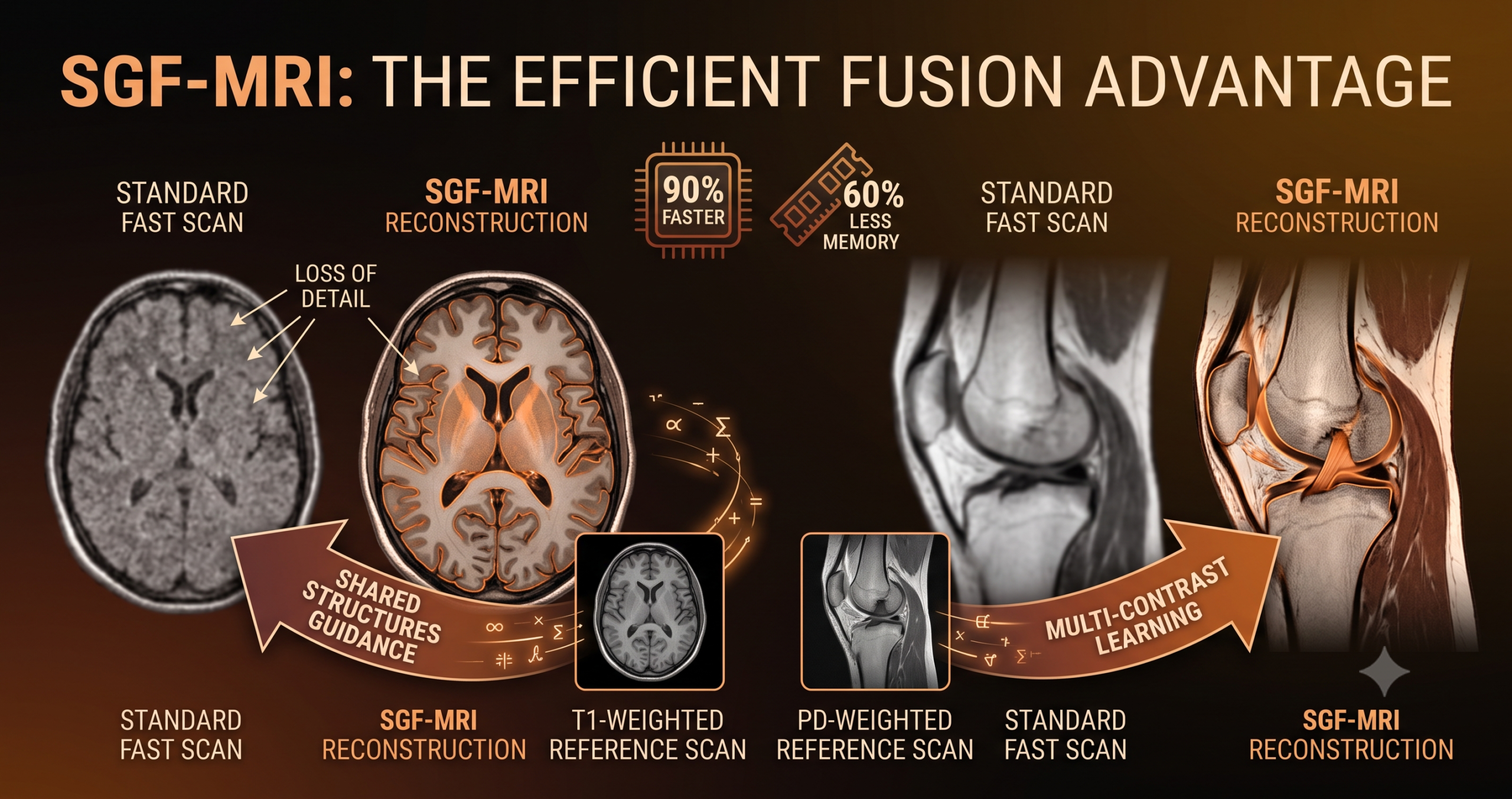
- SGF-MRI uses one fast, fully collected MRI contrast to guide the recovery of a second, undersampled or low resolution contrast of the same anatomy.
- Its core idea, Multi Contrast Structural Distillation, swaps expensive attention math for a lighter neighborhood similarity calculation that scales linearly instead of quadratically.
- On brain and knee datasets the model edges out five published baselines on PSNR and SSIM while cutting inference memory by more than 60 percent and inference time by more than 80 percent against the closest competitor.
- The whole network has about 4 million parameters, similar to the prior leading method and far smaller than transformer heavy alternatives that run into the hundreds of millions.
- The authors tested robustness to small misalignment and to noisy reference scans and found the performance drop in both cases was small.
- This is retrospective research on public datasets, not a validated clinical tool, and the paper itself flags real gaps before anything like this reaches a scanner.
The problem this paper is actually trying to solve
MRI is slow by design. A scanner builds an image by sampling the frequency domain of the body part being imaged, a space researchers call k-space, line by line, and a full sequence can take several minutes. The paper cites earlier clinical work suggesting that motion related to these long acquisitions makes up to a fifth of clinical MRI exams non diagnostic, which is a real cost in repeat scans, delayed diagnoses, and sedated children who have to go through it all over again.
Two engineering tricks try to shrink that time. Super resolution skips the hardware entirely and instead acquires a lower resolution image, then asks a model to fill in detail computationally. Undersampled reconstruction goes further upstream and skips some of the k-space measurements during acquisition itself, relying on an algorithm to recover the missing pieces afterward. Both approaches trade raw acquisition time for computation, and both depend entirely on how well the recovery algorithm can guess what was never directly measured.
Here is where multi contrast imaging becomes interesting rather than just a clinical convenience. A single MRI session routinely produces several contrasts of the same anatomy, T1 weighted, T2 weighted, proton density, and others, because each one highlights different tissue properties. Some of those sequences are quick to fully sample. Others are slow and are the ones radiologists actually want accelerated. If a fast, fully sampled contrast and a slow, undersampled contrast are showing the same knee or the same brain, the fast one already contains a great deal of the structural information the slow one is missing. The trick is fusing that information well, and that is the part most earlier methods got wrong in one of two ways. Either they processed every contrast with an identical network and ignored the relationship between them, or they ran completely separate networks with no information sharing at all.
How earlier multi contrast models tried to fuse information
The lineage here is worth walking through because it explains why SGF-MRI’s design choice is not an arbitrary one. Early work such as DISN concatenated channels from different contrasts and fed them into a densely connected network, which is simple but offers no real mechanism for the model to decide which parts of the reference image are actually useful. rsGAN conditioned its output on low frequency target information and high frequency reference information through fixed channel concatenation, again leaving the fusion rigid rather than learned. Y-Net and MC-PDNet took a similar concatenation route, and DuDoRNet added a recurrent reference branch operating in both spatial and frequency domains, which works but adds training difficulty and computational overhead that scales with the recurrence.
Attention based fusion arrived next and pushed quality higher, at a cost. MCCA used gated channel attention, which captures relationships between feature channels but tends to miss spatial dependencies. MTrans introduced full cross attention between two MRI contrasts, a transformer mechanism whose compute grows quadratically with the number of image positions being compared. DuDoCAF used cross attention restricted to shifted windows to control that cost, and DSFormer mixed k-space operations with a cascaded Swin Transformer. The common thread across nearly all of these is that better fusion quality has historically meant heavier attention computation, and heavier attention computation means slower inference and a bigger memory footprint at exactly the moment a clinical workflow wants speed.
On the super resolution side, a parallel story plays out with reference based methods such as TTSR and MASA-SR, which were built for natural images where the reference picture often shares only a general style with the target rather than the same physical content. Multi contrast MRI super resolution is a friendlier version of that problem because the reference and target are literally the same anatomy, just in a different contrast, which several MRI specific methods exploited through feature concatenation, separable attention in SANet, or dual spatial and channel attention in DCAMSR. The most direct predecessor to this paper is SGSR, a structure guided model that used a co query attention mechanism across spatial and frequency domains. It is worth flagging plainly that SGSR’s first author is the same Shaoming Zheng who leads this new paper. SGF-MRI is not just beating an arbitrary prior state of the art, it is the same research group revisiting their own earlier, heavier design and asking whether a simpler mechanism could match it. That is a more interesting framing than a typical new model paper, because it reads like the authors testing their own assumptions rather than just chasing a leaderboard number.
What SGF-MRI changes, the Multi Contrast Structural Distillation block
SGF-MRI keeps a fairly ordinary convolutional encoder decoder backbone, borrowed from DCAMSR, with three downsampling layers and skip connections, and the decoder actually shares its weights with the encoder rather than learning a separate set. The real contribution sits inside what the authors call the Multi Contrast Structural Distillation block, or MCSD, which is inserted between the encoder and decoder. MCSD runs three operations in sequence on the target and reference feature maps. It first finds which regions of each feature map are structurally important, then measures how similar nearby positions are within and across the two contrasts, and finally fuses that distilled structural signal back into the original image features through attention. The clever part is that the expensive attention computation only happens once, at the fusion step, on a small distilled descriptor, rather than across the entire feature map the way prior transformer based MRI models did it.
Saliency Adaptive Neighborhood, finding where structure actually lives
The first sub module, called Saliency Adaptive Neighborhood or SAN, runs a small convolutional block, a 3 by 3 layer followed by a leaky ReLU and a 1 by 1 layer, over the feature map to estimate how much local structure exists at each position. Smooth tissue regions get a low saliency score, and edges or boundaries between tissue types get a high one. Figure 3 in the paper visualizes this directly on M4Raw brain samples, and the saliency map lights up around the ventricles and cortex, the same regions a basic Sobel edge filter would flag, which is a reassuring sanity check that the learned module is picking up genuine anatomical structure rather than noise. The practical reason this matters is that a fixed, uniform neighborhood wastes computation on homogeneous tissue where there is nothing interesting to recover, while a model that can steer its attention toward edges and boundaries spends its limited capacity where the undersampling artifacts actually need correcting.
Multi Contrast Neighborhood Similarity, the linear time alternative to attention
This is the part that makes the efficiency claims credible rather than aspirational. Instead of computing a full attention map across every pair of positions in the image, which costs quadratic time in the number of pixels, MCNS only compares each token to a small fixed set of neighbors, the two closest tokens in each of the up, down, left, and right directions. That gives linear time complexity in the number of pixels, with the neighborhood size acting as a small constant multiplier rather than a second factor of the image size.
That formula measures how close the feature vector at position j is to a neighboring position k, within the same target contrast, for channel group c, with the comparison scaled by the local variance around position j so the similarity reflects relative contrast rather than absolute pixel intensity. The cross contrast version is structurally identical, it just compares a token in the target contrast to a token in the reference contrast instead.
MCNS computes four of these similarity types in total, target to target, target to reference, reference to target, and reference to reference. The two intra contrast versions help complete missing structure within a single contrast, while the two cross contrast versions are where the actual information transfer between the fast and slow sequences happens. All four get concatenated into one descriptor per position and weighted by the SAN saliency scores from the relevant contrast.
Because genuine anatomical structure such as edges and corners tends to be sparse across an image, while broad intensity shifts are smooth and span large regions, the authors argue the resulting similarity descriptor is itself naturally sparse and concentrated on high frequency content. They exploit that by squeezing the descriptor down with a learned linear projection before it ever reaches the attention step, which keeps the representation compact.
Structures Features Attention, where the fusion finally happens
Only after the structural descriptor has been distilled and squeezed does the model run a single attention operation. The squeezed structural vector becomes the query, while the original encoder feature map supplies the keys and values, a standard scaled dot product attention computed once per decoder stage rather than repeatedly across raw pixels.
The output, F fusion, then merges back into the decoder through the same fusion mechanism DCAMSR used, finishing the reconstruction or super resolution pass. Stacking it all together, structural extraction is cheap and linear, and the one place attention is allowed to run expensively is on a small, already informative descriptor rather than the whole feature map. That ordering is the entire efficiency story in one sentence.
How the experiments were set up
The team evaluated on two public datasets that cover quite different anatomy and acquisition styles. The fastMRI knee dataset uses proton density weighted images to guide fat suppressed proton density weighted images, with 227 subjects for training and 24 held out for testing. The M4Raw brain dataset, a lower field strength dataset, uses T1 weighted scans to guide T2 weighted scans, with 128 subjects for training and 30 for testing. Both reconstruction at 4x and 8x acceleration and super resolution at 2x and 4x upscaling were tested. The encoder decoder backbone used three layers with a downsampling factor of 2 at each stage, and the MCSD block split features into 8 channel groups with a squeezed dimension of 64, a configuration the authors arrived at through their own ablation study rather than picking arbitrarily. Training used a straightforward L1 loss on the target contrast, a batch size of 4, and an initial learning rate of 0.0002 that stepped down by a factor of 10 every 40 epochs. Comparisons were made against MINet, SwinIR, MTrans, DCAMSR, and SGSR, and statistical significance was checked with a paired Wilcoxon signed rank test at a 0.01 threshold, which is a more rigorous bar than simply reporting a higher average score.
What the numbers actually show
SGF-MRI comes out ahead of every baseline on both PSNR and SSIM across both datasets and both tasks, though the margins over the next best method, SGSR, are genuinely modest rather than dramatic. On reconstruction, the gain over SGSR is 0.12 dB at 8x acceleration and 0.08 dB at 4x acceleration on the brain dataset, and 0.07 dB at 8x acceleration on the knee dataset. On super resolution the pattern repeats at a similarly small scale, with gains around 0.03 to 0.08 dB depending on dataset and scale factor. Anyone evaluating this paper for a practical pilot should read those numbers honestly. This is not a model that produces dramatically sharper images than its predecessor, it is a model that produces comparable image quality for a fraction of the compute, and the value proposition is efficiency rather than a quality leap.
| Method | Brain 4x PSNR | Brain 4x SSIM | Brain 8x PSNR | Brain 8x SSIM | Knee 4x PSNR | Knee 8x PSNR |
|---|---|---|---|---|---|---|
| MINet | 29.20 | 0.696 | 27.86 | 0.618 | 29.41 | 28.12 |
| SwinIR | 29.12 | 0.692 | 27.93 | 0.621 | 29.42 | 28.14 |
| MTrans | 27.01 | 0.591 | 25.33 | 0.519 | 27.23 | 25.78 |
| DCAMSR | 29.62 | 0.706 | 28.09 | 0.658 | 29.43 | 28.42 |
| SGSR | 29.74 | 0.714 | 28.15 | 0.663 | 29.60 | 28.43 |
| SGF-MRI | 29.82 | 0.716 | 28.27 | 0.666 | 29.64 | 28.50 |
| Method | Brain 2x PSNR | Brain 4x PSNR | Brain 4x SSIM | Knee 2x PSNR | Knee 4x PSNR | Knee 4x SSIM |
|---|---|---|---|---|---|---|
| MINet | 32.06 | 29.47 | 0.704 | 32.05 | 30.74 | 0.632 |
| SwinIR | 32.16 | 29.73 | 0.709 | 32.01 | 30.59 | 0.628 |
| MTrans | 31.58 | 28.95 | 0.684 | 28.23 | 27.63 | 0.526 |
| DCAMSR | 32.31 | 30.48 | 0.728 | 32.20 | 30.97 | 0.637 |
| SGSR | 32.39 | 30.58 | 0.731 | 32.23 | 31.05 | 0.640 |
| SGF-MRI | 32.42 | 30.62 | 0.731 | 32.26 | 31.13 | 0.641 |
The qualitative figures back up where those small averages actually come from. In the knee scans, the model recovers fine structure around the collateral ligament and the intercondylar fossa more cleanly than the baselines, and in the brain scans the ventricle boundaries and cortical sulci come through with less blur. Those are exactly the small, clinically relevant structures that tend to vanish first under heavy undersampling, so even a modest average PSNR gain can translate into a visibly cleaner small structure in the difference maps the paper includes.
What the ablation study isolates
The authors built up their model piece by piece on the knee dataset at 4x acceleration, and the breakdown is genuinely informative about where the gains come from. A single contrast baseline, essentially ordinary super resolution with no reference image at all, scored 29.37 dB PSNR. Simply adding the reference contrast through the backbone, with no structural distillation yet, pushed that to 29.47 dB, a 0.1 dB gain that on its own justifies the basic premise of multi contrast fusion. Adding intra contrast neighborhood similarity contributed a further 0.07 dB, and adding the cross contrast version on top of that contributed another 0.04 dB, together making up the 0.11 dB gain attributed to MCNS as a whole. Adding the SAN saliency weighting on top of the full model added another 0.03 dB. None of these increments is large in isolation, but they stack in a sensible order, structural similarity matters more than saliency weighting, and within structural similarity, the within contrast signal matters more than the cross contrast signal, which is a fair finding rather than a flattering one for the paper’s main selling point.
A separate hyperparameter sweep tested the number of channel groups used inside MCSD, trying 4, 8, and 16. Four groups under performed, apparently because compressing all the channel information into too few groups loses useful representation capacity. Sixteen groups added computational cost without a meaningful PSNR improvement over 8. The authors settled on 8 as the practical balance, and that is the value used throughout the rest of the paper’s experiments.
The efficiency numbers, and why they are the real headline
This is where the paper earns its keep. Benchmarked on a single NVIDIA RTX 6000 Ada GPU with 48 gigabytes of memory, on 4x super resolution over the fastMRI dataset, SGSR needed 13460 megabytes of inference memory and 0.15 seconds per inference. SGF-MRI needed 4570 megabytes and 0.03 seconds, a reduction of more than 60 percent in memory and more than 80 percent in time against the method it is matching on image quality. The parameter counts tell a similar story from a different angle. SGF-MRI sits at roughly 4 million parameters, in the same range as SGSR, but far below SwinIR and MINet at around 12 million each, and dramatically below MTrans at 746 million parameters.
Robustness checks, and where the cracks start to show
The authors ran two stress tests beyond the standard benchmarks. First, they shifted the reference image by 2 pixels in each of the four cardinal directions during both training and testing, simulating the kind of small patient movement between sequences that happens in nearly every real exam. The resulting PSNR drop was only 0.04 dB, which the authors attribute to the network learning to down weight structural guidance that does not line up well, rather than blindly trusting it.
“Robust to small misalignments common in clinical settings” Zheng, Du, and Qin, Imperial College London, Pattern Recognition 2026
Second, they added Gaussian noise to the reference contrast’s k-space data, with the noise level derived from real background noise estimated in the corners of the images, scaled by a factor of 0.5. The resulting PSNR drop was only 0.02 dB. A separate, less detailed experiment swapped in T1 or T2 weighted scans to guide FLAIR images instead of the original contrast pairing, and the paper reports performance comparable to the prior state of the art without giving exact numbers for that configuration, which is a fair thing to flag as a gap if a reader wanted to scrutinize generalization claims more closely.
Both of the quantified robustness numbers are reassuring, but it is worth being precise about what they do and do not test. A 2 pixel shift and a modest noise injection are small, controlled, synthetic perturbations applied within a benchmark dataset. They are not the same as the kind of misregistration a real clinical exam introduces when a patient repositions between two separate sequences, and the authors are upfront that larger rigid shifts beyond about 5 pixels, and especially the irregular deformations that come from breathing or heartbeat in abdominal or chest imaging, remain a genuine weak point that would need a registration step beforehand.
Clinical translation gap
Strip away the architecture details and the central limitation is simple to state. Every number in this paper comes from retrospectively undersampled public data, meaning fully sampled scans that researchers then artificially degraded by removing k-space lines according to a known mask, then asked the model to reconstruct. That is the standard, reasonable way MRI reconstruction research gets done, and it lets researchers compare models on a level playing field with a known ground truth. It is also, by construction, cleaner than what happens in an actual scanner room. Real clinical degradation includes unpredictable patient motion mid sequence, hardware phase errors, and flow artifacts from blood or cerebrospinal fluid, none of which behave like a clean synthetic undersampling mask.
There is a second, more specific dependency worth naming plainly. The entire method assumes a high quality, fully sampled reference contrast is available to guide the undersampled target contrast. In a clinical protocol where every sequence in the exam is being accelerated to save time, which is often the whole point of speeding up an exam, that assumption can break down, since there may be no clean reference left to lean on. The paper itself lists this as an acknowledged limitation rather than something this article is inferring.
Regulatory and safety notes
None of this is close to a cleared clinical product, and the paper does not claim otherwise. Software that reconstructs or enhances diagnostic medical images typically falls under medical device regulation in most jurisdictions, which in the United States generally means FDA review as software as a medical device, and in the European Union means CE marking under medical device regulation, both of which require evidence well beyond a retrospective benchmark on public research datasets. Before any model in this family could influence an actual diagnostic read, it would need prospective validation against real, not synthetically undersampled, clinical data, ideally across multiple scanner vendors and field strengths, with radiologists blinded to which images came from accelerated reconstruction versus a standard full acquisition.
Where this could matter beyond the two datasets tested
The underlying idea, that a cheap local similarity calculation can substitute for expensive global attention when the two things being compared already share a lot of structure, is not inherently specific to MRI. The same logic could apply to other paired medical imaging problems where one modality or sequence is faster or cheaper than another and the two share anatomy, such as combining a quick localizer scan with a slower diagnostic sequence, or in principle other paired modality problems outside MRI altogether. The authors themselves frame their roadmap modestly, pointing toward extending the approach to 3D and dynamic, that is, time resolved, MRI, and toward testing it on a wider range of contrasts such as T2 star and diffusion weighted imaging, rather than claiming the current 2D, two contrast version is close to done.
Honest limitations
- The model needs a fully sampled, high quality reference contrast, which may not exist in protocols where every sequence is itself being accelerated.
- The architecture is two dimensional and the authors state it faces real challenges scaling to 3D or dynamic, time resolved MRI.
- Generalization to rare pathological tissue such as complex brain tumors, and to other clinically important contrasts like T2 star or diffusion weighted imaging, has not been tested.
- Training relies on an L1 loss, which optimizes pixel level accuracy and can smooth fine texture in ways that may affect perceptual image quality even when PSNR looks favorable.
- Evaluation used 24 held out knee subjects and 30 held out brain subjects, which are reasonable sizes for an academic benchmark but small relative to the population diversity, scanner vendors, and field strengths seen across real hospital networks, and the paper itself calls for further multi center validation.
- All results come from retrospective, synthetically undersampled public datasets rather than prospective clinical data with authentic motion, hardware, and flow artifacts.
Conclusion
The core achievement here is narrower and more honest than a headline grabbing claim of a new best MRI model, and that is precisely what makes it credible. SGF-MRI matches the image quality of the strongest published multi contrast reconstruction and super resolution methods while cutting inference memory by more than 60 percent and inference time by more than 80 percent against its closest competitor, all inside a model with roughly 4 million parameters. The PSNR and SSIM gains over SGSR are real but small, and the paper does not pretend otherwise.
The conceptual shift worth remembering is the deliberate split between where computation should be cheap and where it should be expensive. Earlier multi contrast models tended to run heavy attention everywhere, treating every pixel as potentially relevant to every other pixel. SGF-MRI instead spends its cheap budget on a local, linear time neighborhood similarity calculation across a handful of nearby positions, and reserves the one expensive attention step for fusing an already distilled, already informative structural descriptor back into the image features. That ordering, cheap extraction first, expensive fusion only once and only on compressed information, is a transferable design pattern, not just a one off trick for this particular network.
Whether that pattern travels well beyond two dimensional brain and knee MRI is genuinely unproven. The authors are candid about the boundaries of what they tested, two anatomical regions, two contrast pairings as the primary results, a 2D architecture, and synthetic rather than authentic clinical degradation. Extending the idea to three dimensional or dynamic MRI, to additional contrasts such as T2 star or diffusion weighted sequences, or to other paired imaging problems entirely, are all plausible next steps rather than settled accomplishments.
The honest remaining gap is the one between a strong retrospective benchmark and a tool a radiologist would actually trust during a real exam. Misalignment robustness, noise robustness, and a comparable result on a third contrast pairing are encouraging signs, not proof of clinical readiness, and the paper explicitly calls for prospective validation on real clinical artifacts and multi center data before drawing any conclusion about diagnostic reliability.
What stays with a reader after working through the architecture and the numbers is less about MRI specifically and more about a broader lesson for efficient model design. Matching a more expensive model’s accuracy by being smarter about where you spend computation, rather than simply adding more of it, is a harder and more useful problem to solve than chasing one more fraction of a decibel, and it is the kind of result that quietly changes what becomes deployable rather than what merely tops a leaderboard.
A reference PyTorch implementation
The authors note that code will be released on GitHub, with the repository linked at the end of this article. The implementation below is an independent, educational reconstruction of the architecture described in the paper, written from the method description and equations rather than copied from any released code, intended to make the Saliency Adaptive Neighborhood, Multi Contrast Neighborhood Similarity, and Structures Features Attention modules concrete enough to read and run. It uses simplified synthetic inputs for the smoke test rather than real k-space undersampling logic, since reproducing the exact fastMRI and M4Raw data pipelines is outside the scope of an explainer.
# sgf_mri_reference.py
# Independent educational reimplementation of the SGF-MRI architecture
# Source paper: Zheng, Du, Qin. SGF-MRI. Pattern Recognition 180 (2026) 114188.
# This is not the authors' released code. It exists to make the method readable and runnable.

import math
import torch
import torch.nn as nn
import torch.nn.functional as F


class SaliencyAdaptiveNeighborhood(nn.Module):
    """SAN module. Scores how structurally salient each spatial token is,
    using a small conv stack, per the description in Section 3.3.1."""

    def __init__(self, channels, groups):
        super().__init__()
        self.groups = groups
        self.conv1 = nn.Conv2d(channels, channels, kernel_size=3, padding=1)
        self.act = nn.LeakyReLU(0.1, inplace=True)
        self.conv2 = nn.Conv2d(channels, groups, kernel_size=1)

    def forward(self, feat):
        # feat: (batch, channels, height, width)
        x = self.conv2(self.act(self.conv1(feat)))
        # one saliency scalar per channel group, per spatial position
        saliency = torch.sigmoid(x)
        return saliency  # (batch, groups, height, width)


def _shift(x, dy, dx):
    """Shift a feature map by (dy, dx) with replicate padding, used to read
    a neighbor token at a fixed spatial offset for every position at once."""
    pad = (max(dx, 0), max(-dx, 0), max(dy, 0), max(-dy, 0))
    x_pad = F.pad(x, pad, mode="replicate")
    h, w = x.shape[-2], x.shape[-1]
    top = pad[2] - dy if dy < 0 else 0
    left = pad[0] - dx if dx < 0 else 0
    return x_pad[:, :, top: top + h, left: left + w]


class MultiContrastNeighborhoodSimilarity(nn.Module):
    """MCNS module. Computes group wise exponentially decayed similarity
    between each token and its up, down, left, and right neighbors at
    offset 1 and offset 2, for the four intra and cross contrast pairs,
    matching equations 1 through 4 in the paper."""

    NEIGHBOR_OFFSETS = [(-1, 0), (-2, 0), (1, 0), (2, 0),
                        (0, -1), (0, -2), (0, 1), (0, 2)]

    def __init__(self, channels, groups, squeezed_dim, eps=1e-6):
        super().__init__()
        assert channels % groups == 0
        self.groups = groups
        self.group_dim = channels // groups
        self.eps = eps
        n_neighbors = len(self.NEIGHBOR_OFFSETS)
        distilled_dim = 4 * n_neighbors * groups  # 4 similarity types
        self.squeeze = nn.Linear(distilled_dim, squeezed_dim)

    def _group_similarity(self, feat_a, feat_b, local_var):
        # feat_a, feat_b: (batch, channels, height, width) already grouped
        sims = []
        b, c, h, w = feat_a.shape
        feat_a_g = feat_a.view(b, self.groups, self.group_dim, h, w)
        for dy, dx in self.NEIGHBOR_OFFSETS:
            neighbor = _shift(feat_b, dy, dx)
            neighbor_g = neighbor.view(b, self.groups, self.group_dim, h, w)
            diff_sq = ((feat_a_g - neighbor_g) ** 2).sum(dim=2)  # (b, groups, h, w)
            sim = torch.exp(-diff_sq / (local_var + self.eps))
            sims.append(sim)
        return torch.cat(sims, dim=1)  # (b, groups * n_neighbors, h, w)

    def _local_variance(self, feat):
        # variance of each token relative to its immediate neighborhood,
        # used as sigma_j squared in equations 1 and 2
        mean = F.avg_pool2d(feat, kernel_size=3, stride=1, padding=1)
        sq_mean = F.avg_pool2d(feat ** 2, kernel_size=3, stride=1, padding=1)
        var = (sq_mean - mean ** 2).clamp(min=0)
        return var.mean(dim=1, keepdim=True)

    def forward(self, feat_tar, feat_ref, saliency_tar, saliency_ref):
        var_tar = self._local_variance(feat_tar)
        var_ref = self._local_variance(feat_ref)

        s_tar_tar = self._group_similarity(feat_tar, feat_tar, var_tar)
        s_tar_ref = self._group_similarity(feat_tar, feat_ref, var_tar)
        s_ref_tar = self._group_similarity(feat_ref, feat_tar, var_ref)
        s_ref_ref = self._group_similarity(feat_ref, feat_ref, var_ref)

        n_neighbors = len(self.NEIGHBOR_OFFSETS)
        sal_tar_rep = saliency_tar.repeat_interleave(n_neighbors, dim=1)
        sal_ref_rep = saliency_ref.repeat_interleave(n_neighbors, dim=1)

        s_tar_tar = s_tar_tar * sal_tar_rep
        s_tar_ref = s_tar_ref * sal_ref_rep
        s_ref_tar = s_ref_tar * sal_tar_rep
        s_ref_ref = s_ref_ref * sal_ref_rep

        distilled = torch.cat([s_tar_tar, s_tar_ref, s_ref_tar, s_ref_ref], dim=1)
        b, d, h, w = distilled.shape
        distilled = distilled.permute(0, 2, 3, 1).reshape(b, h, w, d)
        squeezed = self.squeeze(distilled)  # equation 4
        squeezed = squeezed.permute(0, 3, 1, 2)  # back to (b, d_prime, h, w)
        return squeezed


class StructuresFeaturesAttention(nn.Module):
    """SFA module. Uses the distilled structural descriptor as a query
    against the original encoder features, equations 5 and 6."""

    def __init__(self, struct_dim, feat_dim, attn_dim):
        super().__init__()
        self.q_proj = nn.Conv2d(struct_dim, attn_dim, kernel_size=1)
        self.k_proj = nn.Conv2d(feat_dim, attn_dim, kernel_size=1)
        self.v_proj = nn.Conv2d(feat_dim, feat_dim, kernel_size=1)
        self.scale = attn_dim ** -0.5

    def forward(self, structural_feat, image_feat):
        b, _, h, w = image_feat.shape
        q = self.q_proj(structural_feat).flatten(2).transpose(1, 2)  # (b, hw, attn_dim)
        k = self.k_proj(image_feat).flatten(2)                       # (b, attn_dim, hw)
        v = self.v_proj(image_feat).flatten(2).transpose(1, 2)  # (b, hw, feat_dim)
        attn = torch.softmax((q @ k) * self.scale, dim=-1)
        out = attn @ v
        out = out.transpose(1, 2).reshape(b, -1, h, w)
        return out


class MCSDBlock(nn.Module):
    """Full Multi Contrast Structural Distillation block, chaining SAN,
    MCNS, and SFA in the order described in Section 3.3."""

    def __init__(self, channels, groups=8, squeezed_dim=64, attn_dim=32):
        super().__init__()
        self.san_tar = SaliencyAdaptiveNeighborhood(channels, groups)
        self.san_ref = SaliencyAdaptiveNeighborhood(channels, groups)
        self.mcns = MultiContrastNeighborhoodSimilarity(channels, groups, squeezed_dim)
        self.fusion_conv = nn.Conv2d(channels * 2, channels, kernel_size=1)
        self.sfa = StructuresFeaturesAttention(squeezed_dim, channels, attn_dim)

    def forward(self, feat_tar, feat_ref):
        sal_tar = self.san_tar(feat_tar)
        sal_ref = self.san_ref(feat_ref)
        structural = self.mcns(feat_tar, feat_ref, sal_tar, sal_ref)
        fused_feat = self.fusion_conv(torch.cat([feat_tar, feat_ref], dim=1))
        out = self.sfa(structural, fused_feat)
        return out


class ConvBlock(nn.Module):
    def __init__(self, in_ch, out_ch):
        super().__init__()
        self.body = nn.Sequential(
            nn.Conv2d(in_ch, out_ch, 3, padding=1),
            nn.LeakyReLU(0.1, inplace=True),
            nn.Conv2d(out_ch, out_ch, 3, padding=1),
            nn.LeakyReLU(0.1, inplace=True),
        )

    def forward(self, x):
        return self.body(x)


class SGFMRI(nn.Module):
    """Simplified SGF-MRI style network. A shared weight encoder, three
    downsampling stages, an MCSD block bridging encoder and decoder, and
    a decoder that reuses the encoder weights, matching the paper's note
    that the decoder shares weights with the encoder."""

    def __init__(self, base_ch=32, n_layers=3, groups=8, squeezed_dim=64):
        super().__init__()
        self.stem = nn.Conv2d(1, base_ch, 3, padding=1)
        self.shared_blocks = nn.ModuleList([
            ConvBlock(base_ch, base_ch) for _ in range(n_layers)
        ])
        self.downsample = nn.AvgPool2d(2)
        self.upsample = nn.Upsample(scale_factor=2, mode="nearest")
        self.mcsd = MCSDBlock(base_ch, groups=groups, squeezed_dim=squeezed_dim)
        self.decode_merge = nn.Conv2d(base_ch * 2, base_ch, 3, padding=1)
        self.head = nn.Conv2d(base_ch, 1, 3, padding=1)

    def _encode(self, x):
        feats = []
        x = self.stem(x)
        for block in self.shared_blocks:
            x = block(x)
            feats.append(x)
            x = self.downsample(x)
        return feats, x

    def forward(self, target_degraded, reference_full):
        tar_feats, tar_bottleneck = self._encode(target_degraded)
        ref_feats, ref_bottleneck = self._encode(reference_full)

        fused = self.mcsd(tar_bottleneck, ref_bottleneck)

        x = fused
        for block, skip in zip(reversed(self.shared_blocks), reversed(tar_feats)):
            x = self.upsample(x)
            x = self.decode_merge(torch.cat([x, skip], dim=1))
            x = block(x)

        out = self.head(x)
        return out


def reconstruction_loss(pred, target):
    """The paper trains with a plain L1 loss on the target contrast."""
    return F.l1_loss(pred, target)


def psnr(pred, target, max_val=1.0):
    mse = F.mse_loss(pred, target).clamp(min=1e-10)
    return 10 * torch.log10((max_val ** 2) / mse)


def ssim(pred, target, window_size=11, c1=0.01 ** 2, c2=0.03 ** 2):
    """Compact single scale SSIM using a Gaussian window, for evaluation."""
    coords = torch.arange(window_size, dtype=torch.float32) - window_size // 2
    g = torch.exp(-(coords ** 2) / (2 * 1.5 ** 2))
    g = (g / g.sum()).unsqueeze(0)
    window = (g.t() @ g).unsqueeze(0).unsqueeze(0)
    window = window.to(pred.device)

    pad = window_size // 2
    mu_p = F.conv2d(pred, window, padding=pad)
    mu_t = F.conv2d(target, window, padding=pad)
    mu_p_sq, mu_t_sq, mu_pt = mu_p ** 2, mu_t ** 2, mu_p * mu_t

    sigma_p_sq = F.conv2d(pred * pred, window, padding=pad) - mu_p_sq
    sigma_t_sq = F.conv2d(target * target, window, padding=pad) - mu_t_sq
    sigma_pt = F.conv2d(pred * target, window, padding=pad) - mu_pt

    ssim_map = ((2 * mu_pt + c1) * (2 * sigma_pt + c2)) / (
        (mu_p_sq + mu_t_sq + c1) * (sigma_p_sq + sigma_t_sq + c2)
    )
    return ssim_map.mean()


def train_one_epoch(model, loader, optimizer, device):
    model.train()
    running_loss = 0.0
    for target_degraded, reference_full, target_full in loader:
        target_degraded = target_degraded.to(device)
        reference_full = reference_full.to(device)
        target_full = target_full.to(device)

        optimizer.zero_grad()
        pred = model(target_degraded, reference_full)
        loss = reconstruction_loss(pred, target_full)
        loss.backward()
        optimizer.step()
        running_loss += loss.item()
    return running_loss / len(loader)


def evaluate(model, loader, device):
    model.eval()
    total_psnr, total_ssim, n = 0.0, 0.0, 0
    with torch.no_grad():
        for target_degraded, reference_full, target_full in loader:
            target_degraded = target_degraded.to(device)
            reference_full = reference_full.to(device)
            target_full = target_full.to(device)
            pred = model(target_degraded, reference_full).clamp(0, 1)
            total_psnr += psnr(pred, target_full).item()
            total_ssim += ssim(pred, target_full).item()
            n += 1
    return total_psnr / n, total_ssim / n


def smoke_test():
    """Runs a forward and backward pass on random dummy data to confirm
    the architecture is wired correctly end to end."""
    device = torch.device("cuda" if torch.cuda.is_available() else "cpu")
    model = SGFMRI(base_ch=16, n_layers=3, groups=4, squeezed_dim=32).to(device)
    optimizer = torch.optim.Adam(model.parameters(), lr=2e-4)
    scheduler = torch.optim.lr_scheduler.StepLR(optimizer, step_size=40, gamma=0.1)

    batch, h, w = 2, 64, 64
    target_degraded = torch.rand(batch, 1, h, w, device=device)
    reference_full = torch.rand(batch, 1, h, w, device=device)
    target_full = torch.rand(batch, 1, h, w, device=device)

    pred = model(target_degraded, reference_full)
    assert pred.shape == target_full.shape, "output shape mismatch"

    loss = reconstruction_loss(pred, target_full)
    loss.backward()
    optimizer.step()
    scheduler.step()

    with_grad_psnr = psnr(pred.detach().clamp(0, 1), target_full)
    with_grad_ssim = ssim(pred.detach().clamp(0, 1), target_full)

    print(f"smoke test passed, output shape {pred.shape}")
    print(f"dummy loss {loss.item():.4f}")
    print(f"dummy psnr {with_grad_psnr.item():.2f} dB, dummy ssim {with_grad_ssim.item():.4f}")


if __name__ == "__main__":
    smoke_test()
Running that script end to end on random tensors confirms the shapes line up through the encoder, the MCSD block, and the weight sharing decoder, which is the same wiring described in the paper even though the dummy data here carries no real anatomical structure for the model to learn from.
Frequently asked questions
What does SGF-MRI actually do
It is a deep learning model that recovers a high quality MRI image of one contrast, such as a T2 weighted brain scan, by borrowing structural information from a second, faster contrast of the same body part, such as a T1 weighted scan, that was already fully collected during the same exam.
How is SGF-MRI different from earlier multi contrast MRI models
Earlier attention based models compared every image position to every other image position, which gets expensive as images get larger. SGF-MRI instead compares each position only to a small set of nearby neighbors using a lightweight similarity calculation, then runs one cheaper attention step at the end to fuse that distilled structural information with the image features.
Does SGF-MRI need two full MRI scans to work
It needs one fully sampled reference contrast and one undersampled or low resolution target contrast of the same anatomy. If every sequence in an exam is being accelerated at once, there may be no clean reference contrast left, which the paper lists as a real limitation.
How much faster or lighter is SGF-MRI compared to other models
On the benchmark reported in the paper, SGF-MRI used about 4570 megabytes of inference memory and 0.03 seconds per inference, against 13460 megabytes and 0.15 seconds for the prior leading method, while reaching similar or slightly better PSNR and SSIM scores.
Has SGF-MRI been tested in real hospitals yet
No. The results in the paper come from retrospective experiments on public research datasets with synthetic undersampling, not from prospective clinical trials, and the authors explicitly call for further validation on real clinical data before any claim about diagnostic reliability.
Can SGF-MRI work with contrasts other than T1 and T2
The main experiments use T1 guiding T2 for brain imaging and proton density guiding fat suppressed proton density for knee imaging. The authors report a supplementary experiment using T1 or T2 to guide FLAIR images with comparable results, but generalization to contrasts such as T2 star or diffusion weighted imaging has not yet been tested.
Read the full method, the supplementary robustness experiments, and the released code for yourself.
You can also read the open access paper directly on Pattern Recognition for the full supplementary material, including the FLAIR guidance experiment and the effect size analysis the authors mention but keep out of the main tables.