
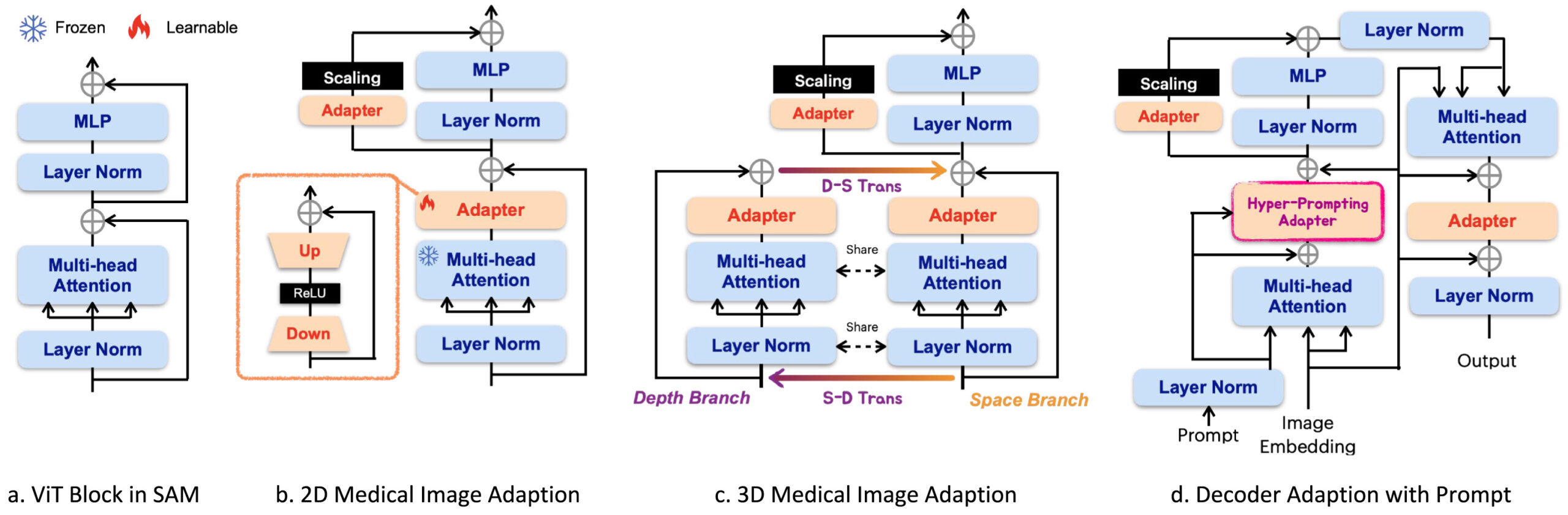
Fully retraining a billion parameter foundation model every time it stumbles on a new domain is expensive, slow, and risks quietly erasing the very generality that made the model useful in the first place. A team spanning the National University of Singapore, the University of Alberta, A*STAR, and Carnegie Mellon took a narrower bet on the Segment Anything Model instead. Rather than fine tuning SAM’s roughly 636 million parameters on medical scans, they froze essentially all of them and inserted small trainable adapter modules at specific points in the network, touching only about 13 million parameters, a bit over 2 percent of the total. Their paper, published in Medical Image Analysis in March 2025, reports this small addition beating a fully fine tuned version of SAM called MedSAM across 17 different segmentation tasks spanning five imaging modalities.
Key points
- Med-SA inserts lightweight bottleneck adapters into SAM’s encoder and decoder while keeping the original pretrained SAM weights completely frozen.
- A component called Space-Depth Transpose lets the same 2D attention blocks handle 3D volumes like CT and MRI by processing spatial and depth correlations in two separate passes that get added together.
- A second component called the Hyper-Prompting Adapter uses the user’s click or box prompt to generate weights that reshape the adapter’s own features, so the adaptation itself responds to what the clinician is pointing at.
- On the BTCV abdominal CT benchmark, Med-SA reaches 89.8 percent average Dice while updating only 13 million parameters, ahead of Swin-UNetr’s 86.9 percent with 138 million tunable parameters and ahead of fully fine tuned MedSAM’s 80.4 percent with 636 million tunable parameters.
- Med-SA degrades far less than other SAM variants when the prompt itself is imprecise, which the paper attributes directly to the adapter learning task specific semantic regions rather than relying purely on prompt geometry.
- The paper’s own failure case section shows the model struggling with genuinely ambiguous prompts, such as a bounding box that necessarily captures two adjacent organs at once.
The problem with two extremes
When a general purpose model like SAM meets a specialized domain like radiology, there are really only two conventional options, and the paper frames its contribution as a rejection of both. The first option is to use SAM exactly as released, prompting it with a box or a click the way you would on a natural photograph. The paper cites earlier studies showing this reaches noticeably subpar results on medical images, and the underlying reason is straightforward. SAM’s training data taught it what object boundaries look like in ordinary photographs, and medical images routinely violate the assumptions that training baked in, with low contrast between tissue types, boundaries that fade rather than snap into focus, and lesions that can be only a few pixels across.
The second option is full fine tuning, training every one of SAM’s parameters on medical data until the whole network internalizes the new domain. MedSAM, an earlier and influential effort along these lines, does exactly this. The paper argues this approach is costly in both computation and memory, and raises a more subtle concern too, questioning whether full fine tuning is even necessary given that prior research on transfer learning has repeatedly shown pretrained visual models already transfer reasonably well to medical images without needing every weight disturbed. Full fine tuning also carries a real risk, since retraining the entire network on a comparatively narrow medical dataset can overwrite general visual knowledge the model spent enormous compute learning in the first place, a phenomenon usually called catastrophic forgetting.
Med-SA is built as a middle path between these extremes, borrowed from a technique with a long track record in natural language processing called Adaptation, sometimes shortened to Adaption in the paper’s own terminology. The idea is to insert small bottleneck modules at specific points inside a frozen network and train only those modules, leaving the original pretrained weights untouched. This has worked well for adapting large language models to new tasks, but the authors point out that applying the same idea to an interactive vision model like SAM is not a solved problem, for two specific reasons that shape the rest of the paper’s design choices.
Why medical images and SAM’s interface both resist a naive adapter
The first complication is dimensionality. Natural images are two dimensional, and so is SAM’s entire architecture. Medical imaging, though, frequently involves three dimensional volumes, CT and MRI scans built from dozens or hundreds of stacked slices where the correlation between adjacent slices carries real diagnostic information. Simply running SAM slice by slice through a volume, which is the naive approach, throws away that volumetric context entirely, treating each slice as an independent 2D problem even though a tumor or organ boundary should look coherent as it grows and shrinks across neighboring slices.
The second complication is specific to SAM’s interactive design. Unlike a typical image classifier, SAM does not just take an image and produce an output, it takes an image plus a prompt, a point, a box, or a mask that tells it what to segment. Adapter research in NLP and even most adapter research in computer vision was not built around this kind of prompt conditioned interaction. The paper notes that how to meaningfully incorporate a user’s prompt into a small adapter module, rather than just adapting the raw image features, was essentially unexplored territory before this work. Both of these gaps get a dedicated architectural answer, Space-Depth Transpose for the dimensionality problem and the Hyper-Prompting Adapter for the prompt integration problem.
How the adapter itself is built
Before getting to the two novel components, it helps to understand the basic adapter Med-SA inserts throughout SAM’s frozen backbone. Each adapter is a simple bottleneck, a down projection that compresses the incoming embedding into a smaller dimension, a ReLU activation, and an up projection that expands it back to the original size. This is a well established, lightweight pattern precisely because the bottleneck keeps the parameter count low relative to the full sized layers it sits alongside.
Placement matters as much as the adapter’s internal design. In SAM’s encoder, which is built from a stack of standard Vision Transformer blocks, Med-SA places two adapters in every block, one immediately following the multi head self attention layer and a second positioned in the residual path of the MLP layer that comes after. The authors are explicit about why both locations matter rather than just one. Multi head attention is what lets a Vision Transformer capture relationships across different parts of an image, both nearby and distant, so adapting right after attention is an obvious place to inject task specific behavior. But the paper also draws on separate research showing that a transformer’s MLP sublayers matter more than commonly assumed, since without them a stack of pure attention layers tends toward degenerate, low rank representations. Placing adapters on both the attention output and the MLP residual path, running in parallel to the frozen branch rather than replacing it, lets task specific features complement the general features SAM already learned rather than overwrite them. A scaling factor, denoted s, controls how strongly the adapter branch’s contribution gets weighted against the frozen branch, and the paper’s own hyperparameter search, discussed further below, found a fairly small value of 0.05 worked best.
The decoder gets a slightly richer treatment, with three adapters per Vision Transformer block rather than two, because the decoder is where the prompt actually enters the computation. The first decoder adapter is specifically responsible for integrating the prompt embedding, and this is where the Hyper-Prompting Adapter design lives. The second decoder adapter mirrors the encoder’s MLP adapter placement. The third sits after the residual connection following the cross attention between image embeddings and the prompt, with its own residual connection and layer normalization closing out the block before producing the final output.
Space-Depth Transpose, teaching 2D attention to see in 3D
The core insight behind SD-Trans is that a single attention operation can be run twice on the same data, once organized to capture spatial relationships within a slice and once organized to capture depth relationships across slices, and the two results can simply be added together. For a 3D input with depth D, the space branch takes an input shaped D by N by L, where N is the number of embeddings per slice and L is the embedding length, and treats D as a batch dimension, running attention over the N by L spatial arrangement within each of the D slices independently. That captures the usual within slice spatial correlations a 2D attention block would normally learn.
The depth branch takes the exact same underlying data and transposes it into an N by D by L arrangement instead, so now the attention operation runs over D by L for each of the N spatial positions, meaning it is comparing the same spatial location across every slice in the volume rather than comparing different spatial locations within one slice. This is the piece that captures volumetric, cross slice correlation. Critically, both branches reuse the exact same attention weights, since the SAM backbone stays frozen either way, only the way the input tensor gets reshaped before entering that shared attention operation differs between the two branches. After the depth branch computes its result, it gets transposed back to its original shape and added directly to the space branch’s output, folding the depth information into the final representation. The paper explicitly tested two more elaborate ways to combine the space and depth branch outputs, concatenation and a learned cross attention fusion, and found in an ablation study that cross attention edged out simple addition by less than a percentage point of Dice score while adding 28.3 million extra parameters, more than double the entire adapter’s parameter budget. The authors chose plain addition as the default specifically to preserve the lightweight design philosophy the whole method is built around, a reasonable trade off given how small the accuracy gain from the heavier fusion method actually was.
Hyper-Prompting Adapter, letting the prompt reshape the adapter itself
The second architectural contribution addresses a subtler problem. A typical adapter transforms whatever features flow through it the same way regardless of context. But in an interactive segmentation model, the user’s prompt is not incidental information, it is the entire point, telling the network which of potentially many structures in the image it should be segmenting right now. The paper’s answer is to let the prompt embedding directly generate the weights the adapter uses, rather than treating the prompt as just another input to be processed alongside the image.
Concretely, the prompt information, whether that is a click location, a click’s foreground or background label, or a bounding box location, gets concatenated and compressed into a prompt embedding. That embedding is then passed through a small MLP and reshaped into an actual weight tensor, written in the paper as
where Re denotes the reshape operation and M denotes the MLP doing the projection. The MLP maps the prompt embedding from a compact N by L shape up to N by the product of an input length and an output length, then that gets reshaped from a flat one dimensional embedding into an actual two dimensional weight matrix per query, shaped N by L-in by L-out. That weight matrix is then applied directly to the adapter’s own down projected embedding through a matrix product
with a normalization step along the length dimension before the ReLU activation. The whole process repeats across three stacked hyper prompting layers, each with its own individually projected weight set. The practical effect is that the adapter’s transformation is not fixed, it is conditioned on exactly where the user pointed or boxed, which lets the same adapter module behave differently depending on which organ or lesion a clinician is currently indicating, all while adding comparatively few extra parameters relative to what it would cost to generate an entirely separate network conditioned on the prompt.
Why the ablation study on this component is the paper’s strongest evidence
The authors test three ways of getting prompt information into the adapter, simple element wise addition, concatenation, and the full Hyper-Prompting Adapter. Addition and concatenation both help over a baseline with no prompt conditioning at all, but the improvements are described as marginal. The Hyper-Prompting Adapter produces what the paper calls a significant enhancement on top of that. This matters because it shows the benefit is not just from getting prompt information into the adapter somehow, it specifically comes from letting the prompt reshape the adapter’s transformation dynamically, rather than simply appending prompt information as extra input features.
What the results actually show
The headline BTCV comparison
The paper’s central benchmark is BTCV, a widely used abdominal CT dataset with 12 anatomical structures annotated across 50 subjects and 1463 axial slices. Comparing against well established, purpose built segmentation architectures rather than other SAM variants first gives a sense of where Med-SA lands relative to the field’s existing best methods.
| Model | Tunable params (M) | Average Dice | HD95 (lower is better) |
|---|---|---|---|
| TransUNet | 37 | 83.8% | 8.12 |
| UNetr | 104 | 85.6% | 6.35 |
| Swin-UNetr | 138 | 86.9% | 5.85 |
| nnUNet | 16 | 80.2% | 23.49 |
| CoTr | 41.9 | 85.0% | 6.12 |
| TransUNet3D | 41.4 | 85.6% | 6.44 |
| Med-SA, automatic everything | 13 | 88.1% | 3.38 |
| Med-SA, 1 point prompt | 13 | 88.3% | 3.22 |
| Med-SA, 3 point prompts | 13 | 88.7% | 3.06 |
| Med-SA, box prompt at 75% overlap | 13 | 89.8% | 2.18 |
Med-SA’s best configuration beats Swin-UNetr, the strongest specialized architecture in this comparison, by 2.9 percentage points of Dice while using roughly a tenth as many tunable parameters, 13 million against 138 million. Even Med-SA’s fully automatic mode, run without any human prompt at all in a segment everything setting analogous to vanilla SAM’s automatic mode, still edges out Swin-UNetr by 1.2 points. Against methods purpose built for volumetric data specifically, CoTr and TransUNet3D, Med-SA’s box prompted result beats both by 4 to 5 percentage points of Dice.
Beating a fully fine tuned SAM with 2 percent of its parameters
The more pointed comparison sits against other ways of adapting SAM itself, including MedSAM, which represents the full fine tuning approach the paper positions itself against directly. Across every prompt setting tested, Med-SA outperforms MedSAM’s 636 million tunable parameters using only 13 million of its own, roughly 2 percent as many. At the box prompt 75 percent overlap setting, Med-SA reaches 89.8 percent Dice against MedSAM’s 80.4 percent, a gap of nearly 9.5 percentage points despite MedSAM having updated every single one of SAM’s weights on medical data. The paper also compares against a wide range of other SAM adaptation attempts, including SAMed, SAM-Med2D, SAM-U, and several 3D specific SAM variants like SAM3D, 3DSAM-adt, MA-SAM, Promise, and SAM-Med3D, and Med-SA comes out ahead of SAM-Med3D specifically, the strongest of these 3D competitors, by 0.7 points of Dice, 2.0 points of IoU, and 1.64 on the HD95 boundary metric, while remaining notably more stable across different prompt settings than most of the alternatives.
One detail worth sitting with, since it is easy to read past in a results table, vanilla zero shot SAM performs poorly on this benchmark across every prompt type tested, with Dice scores in the 44 to 63 percent range depending on prompt quality, far below any of the fine tuned or adapted alternatives. The paper is candid that this comparison might look unfair given SAM was never trained for medical images specifically, but frames the gap as direct confirmation that some form of medical specific adaptation, whether full fine tuning or a lightweight adapter, is genuinely necessary rather than optional for this domain.
Generalizing across five different imaging modalities
Beyond the 3D CT benchmark, the paper tests Med-SA across four additional segmentation tasks spanning very different imaging modalities, retinal fundus photography for optic disc and cup segmentation, brain MRI for glioblastoma subregions, ultrasound for thyroid nodules, and dermoscopic photography for melanoma.
| Task and modality | Best specialized or general method | Med-SA, box 75% |
|---|---|---|
| Optic disc, fundus photo | CoTr, 95.8% Dice | 98.3% Dice |
| Optic cup, fundus photo | CoTr, 85.9% Dice | 87.5% Dice |
| Brain tumor, MRI | TransUNet3D, 88.9% Dice | 90.5% Dice |
| Thyroid nodule, ultrasound | UltraUNet, 84.5% Dice | 88.4% Dice |
| Melanoma, dermoscopy | BAT, 91.2% Dice | 93.0% Dice |
The pattern the paper highlights here is that task specific specialized models, the kind purpose built and tuned for exactly one modality, frequently top the leaderboard on their home turf but fall behind noticeably when applied to a different modality. UltraUNet, for instance, achieves the strongest thyroid nodule result among the specialized baselines but performs comparatively poorly on optic disc segmentation. Med-SA’s single, shared architecture matches or beats the best specialized method on every one of these five tasks simultaneously, which is a genuinely different kind of claim than simply winning on one benchmark, since it argues for one adaptable backbone rather than five separately engineered networks.
Looking at other SAM based interactive methods across these same modalities, vanilla zero shot SAM fails outright on a meaningful share of cases for optic disc, optic cup, and thyroid nodule segmentation, with the paper reporting results omitted entirely because the algorithm failed on more than 70 percent of samples for those tasks. That is a stronger statement than merely underperforming, it points to SAM sometimes not producing a usable segmentation at all on these structures without adaptation, which underscores why the paper treats some form of medical specific tuning as close to mandatory rather than a marginal improvement.
The ablation study that isolates what actually matters
The paper runs a careful component removal study specifically to attribute Med-SA’s gains to SD-Trans and HyP-Adpt individually rather than crediting the overall adapter idea in general.
| Configuration | BTCV average Dice |
|---|---|
| Baseline, SAM plus plain adapter, no SD-Trans, no prompt conditioning | 79.3% |
| Add SD-Trans | 84.7% |
| SD-Trans plus simple addition prompt conditioning | 86.1% |
| SD-Trans plus concatenation prompt conditioning | 86.4% |
| SD-Trans plus full Hyper-Prompting Adapter, complete Med-SA | 88.3% |
Adding SD-Trans alone lifts the baseline by 5.4 percentage points, confirming that treating volumetric correlation explicitly matters a great deal for 3D data, since the baseline here processes each slice independently despite the data being inherently three dimensional. Layering in prompt conditioning through the full Hyper-Prompting Adapter adds another meaningful 2.2 points on top of the simpler addition based prompt conditioning, which itself only added 1.4 points over no prompt conditioning at all. The two components are clearly doing distinct, complementary work rather than one accounting for nearly all the improvement.
What happens to adapter rank, layer placement, and the scaling factor
A separate set of experiments investigates the internal hyperparameters of the adapter bottleneck itself. Sweeping the adapter’s internal rank, essentially the width of its compressed bottleneck dimension, shows accuracy climbing from 75.2 percent Dice with a rank of just 1, up through 85.6 percent at rank 16 and 86.9 percent at rank 32, reaching 88.3 percent at rank 64 where performance saturates, and then actually declining slightly to 87.8 percent at rank 256, suggesting the adapter can be given too much capacity and starts overfitting rather than continuing to improve. Layer placement tells an interesting story too. Inserting adapters only into the top half of the network’s layers, layers 17 through 32, produced roughly 9 percentage points higher Dice than inserting the same number of adapters into the bottom half, layers 1 through 16, which suggests the deeper, more semantically rich layers of the frozen backbone benefit more from task specific adaptation than the shallower layers closer to raw pixel input.
The scaling factor s, which balances how strongly the adapter branch’s output gets weighted against the frozen branch’s output, turned out to have a fairly narrow sweet spot around 0.05, with both smaller values around 0.01 and larger values around 0.10 to 0.20 performing worse. The authors note this is a smaller value than what has typically worked best in NLP adapter research, and offer training stability as the likely explanation, arguing that SAM’s already strong, broadly trained segmentation ability can be destabilized by leaning too heavily on the newly initialized, still learning adapter branch during early training if that branch’s contribution is weighted too aggressively.
Robustness to imprecise prompts, a genuinely useful finding
One of the more clinically relevant results in the paper concerns what happens when the prompt itself is not perfectly accurate, which is the realistic scenario in a busy clinical workflow rather than the idealized ground truth boxes used in many benchmark comparisons. The paper compares performance at the box prompt 75 percent overlap setting against the sloppier 50 percent overlap setting across several models. Vanilla SAM’s average Dice on BTCV drops by 11.0 percentage points between these two prompt qualities, SAMed drops by 14.4 points, and fully fine tuned MedSAM drops by 11.2 points. Med-SA’s own drop across that same prompt degradation, from 89.8 percent down to 87.6 percent, is only about 2.2 points, a noticeably smaller decline than any of the comparison methods. The authors attribute this specifically to the task specific adapter learning to recognize the correct anatomical region on its own, reducing how heavily the model depends on the prompt being drawn with precision in the first place. That is a meaningfully different and arguably more clinically important claim than simply reporting a higher accuracy number under ideal conditions, since real clinicians drawing boxes quickly during a busy workflow will not always draw them with textbook precision.
What real clinicians do differently from synthesized prompts
A smaller but notable experiment brought three senior ophthalmologists, each with more than a decade of clinical experience, into the evaluation directly, having them provide live click prompts for optic cup segmentation and comparing those against the paper’s own synthesized, algorithmically generated click prompts. The result carries a small but genuine surprise. With just a single click, the synthesized prompts actually performed slightly better than the real clinicians’ clicks. But as more clicks were added, three, five, seven, and nine, the human generated prompts pulled ahead and stayed ahead. The authors’ explanation is intuitive once stated, humans tend to place a first click near the center of the structure they want segmented, which conveys relatively little information about where the true boundary actually sits, but subsequent clicks tend to land specifically on ambiguous edges, offering the kind of detailed boundary information a randomly synthesized click sampling strategy would not systematically target. The practical takeaway the authors draw is that around three clicks may represent a reasonable balance point for real world clinical use, enough to capture the boundary detail human intuition provides without demanding an excessive number of interactions from a busy clinician.
Clinical translation gap
Despite the breadth of this evaluation, spanning 17 tasks and five modalities, there is still real distance between these results and deployment in an actual radiology or ophthalmology workflow. Every dataset used here is a publicly available research benchmark, BTCV, REFUGE2, BraTS2021, a mixed thyroid ultrasound set, and ISIC2019, each collected under its own protocol at its own set of institutions, and the paper reports results using each dataset’s own default training, validation, and test split rather than testing generalization to entirely new hospitals, scanners, or patient populations beyond what those default splits already capture. The clinician comparison study, while a welcome and unusually direct piece of real world validation, involved only three ophthalmologists on a single task, optic cup segmentation, and should be read as an interesting pilot observation about prompting behavior rather than a broad claim about clinical usability across all 17 tasks the paper covers. No study in the paper measures how Med-SA’s segmentations would actually change a diagnosis, a treatment plan, or a clinical outcome, since Dice score and Hausdorff distance are geometric accuracy measures against a reference annotation, not measures of clinical utility or patient benefit. Any real deployment would require prospective validation against clinical decision making, formal regulatory clearance appropriate to the specific intended use, and testing across the kind of imaging equipment and patient diversity a single research benchmark cannot fully represent.
Key takeaway
The paper’s honest failure case section is arguably its most valuable contribution for anyone considering building on this work. Med-SA cannot resolve genuine prompt ambiguity, if a bounding box necessarily contains two adjacent anatomical structures because they sit close together, the model segments every plausible candidate and leaves the final choice to the user. That is a sensible fallback behavior, but it is also a reminder that no amount of adapter engineering removes the fundamental limitation that a prompt based system is only as unambiguous as the prompt itself.
Honest limitations
Beyond the deployment gap already discussed, a few other constraints are worth stating directly. The paper’s own failure case analysis, illustrated with a pancreas segmentation example where a bounding box tight enough to capture the pancreas necessarily also captures the adjacent aorta, shows Med-SA responding by segmenting all plausible organs within the ambiguous prompt region rather than confidently picking one, which the authors themselves describe as potentially cumbersome for the end user in exactly the situations where clean, single answer segmentation would matter most. The proposed fix, extending the prompt vocabulary to include scribbles or text descriptions, is listed as future work rather than something the current paper implements or tests.
The comparison against MedSAM-2, a newer competitor built on the SAM2 backbone using full fine tuning with a video style single prompt approach, is genuinely mixed rather than a clean win for Med-SA. MedSAM-2 actually surpasses every prompt setting of Med-SA on the 3D BTCV dataset except the box prompt 75 percent overlap setting, while requiring dramatically fewer prompts overall since it treats a whole 3D volume as a video clip needing only one initial prompt rather than Med-SA’s per slice prompting requirement. The authors are upfront that this suggests real promise in applying their own adapter techniques to a SAM2 style backbone as future work, rather than claiming Med-SA is simply superior in every dimension to every possible competitor.
Finally, several of the paper’s strongest claims rest on comparisons using each method’s own reported settings and the paper’s own reproduction of comparison baselines using their default configurations, which is standard practice in this kind of benchmark study but does mean the exact numbers for competing methods could shift somewhat under different reproduction efforts or hyperparameter tuning by other research groups. The five repeated trials reported to measure variance from prompt randomness are a genuinely good practice and do show small standard deviations, generally under one percentage point of Dice, which supports the stability of the specific numbers reported, though this measures consistency of Med-SA’s own results rather than addressing reproducibility of the baseline comparisons.
Where this points next
The core idea that transfers most readily beyond this specific paper is the general strategy of solving a domain adaptation problem with a small, purpose designed module rather than reaching for full fine tuning by default. SD-Trans in particular is a clean, almost elegant solution to a genuinely common problem, any 2D vision foundation model that needs to handle 3D data could plausibly borrow the same space and depth branch splitting trick without needing a fundamentally different architecture. The Hyper-Prompting Adapter’s core idea, letting auxiliary conditioning information reshape an adapter’s own weights rather than just concatenating that information as extra input, is similarly general and could extend to other conditioning signals beyond spatial prompts, text descriptions or patient metadata come to mind as plausible candidates worth testing. The authors’ own stated next step, applying adapter techniques to the newer MedSAM-2 and SAM2 style video backbone, is a sensible priority given how competitive MedSAM-2 already proved on the 3D benchmark despite requiring far more parameters to update.
Complete PyTorch implementation
The following is a full, runnable reproduction of the Med-SA style adapter block described in the paper, including the bottleneck adapter itself, the Space-Depth Transpose attention module, the Hyper-Prompting Adapter, a ViT block wrapper showing where the adapters attach, a training loop, an evaluation function using Dice score, and a smoke test on random dummy data so you can confirm the shapes work end to end before attaching this to a real frozen SAM checkpoint.
# med_sa_adapter.py
# A runnable reproduction of the core Med-SA adapter components from
# Wu, Wang, Hong, Ji, Fu, Xu, Xu, Jin, "Medical SAM adapter,"
# Medical Image Analysis, 2025.
# This models the Adapter bottleneck, Space-Depth Transpose (SD-Trans),
# and the Hyper-Prompting Adapter (HyP-Adpt). It is designed to sit
# alongside a frozen SAM ViT block, not to reimplement SAM itself.

import torch
import torch.nn as nn
import torch.nn.functional as F
from torch.utils.data import Dataset, DataLoader


# ---------------------------------------------------------------------
# The basic bottleneck adapter, down-projection, ReLU, up-projection
# ---------------------------------------------------------------------
class Adapter(nn.Module):
    def __init__(self, dim, rank=64, scale=0.05):
        super().__init__()
        self.down = nn.Linear(dim, rank)
        self.up = nn.Linear(rank, dim)
        self.scale = scale
        nn.init.zeros_(self.up.weight)   # start as a near no-op so the frozen branch dominates early
        nn.init.zeros_(self.up.bias)

    def forward(self, x, external_weight=None):
        h = F.relu(self.down(x))
        if external_weight is not None:
            # used by HyP-Adpt to reshape the adapter's own bottleneck features
            h = F.relu(F.layer_norm(torch.bmm(h, external_weight), h.shape[-1:]))
        return x + self.scale * self.up(h)


# ---------------------------------------------------------------------
# Space-Depth Transpose, runs the same attention over spatial
# correlations and over depth correlations, then adds the results
# ---------------------------------------------------------------------
class SDTrans(nn.Module):
    def __init__(self, dim, num_heads=8):
        super().__init__()
        # a single shared attention module used for both branches, matching
        # the paper's design of reusing the same weights for space and depth
        self.attn = nn.MultiheadAttention(dim, num_heads, batch_first=True)

    def forward(self, x):
        # x: B x D x N x L  (batch, depth/slices, spatial tokens, embed dim)
        B, D, N, L = x.shape

        # space branch: treat D as part of the batch, attend over N tokens per slice
        space_in = x.reshape(B * D, N, L)
        space_out, _ = self.attn(space_in, space_in, space_in)
        space_out = space_out.view(B, D, N, L)

        # depth branch: transpose so attention runs over the D slices per spatial token
        depth_in = x.permute(0, 2, 1, 3).reshape(B * N, D, L)
        depth_out, _ = self.attn(depth_in, depth_in, depth_in)
        depth_out = depth_out.view(B, N, D, L).permute(0, 2, 1, 3)

        return space_out + depth_out


# ---------------------------------------------------------------------
# Hyper-Prompting Adapter, the prompt embedding generates a weight
# tensor that is applied to the adapter's own down-projected features
# ---------------------------------------------------------------------
class HyperPromptingAdapter(nn.Module):
    def __init__(self, dim, rank=64, prompt_dim=256, num_layers=3, scale=0.05):
        super().__init__()
        self.rank = rank
        self.num_layers = num_layers
        self.adapter = Adapter(dim, rank=rank, scale=scale)
        # one small MLP per hyper-prompting layer, each projects the prompt
        # embedding into a rank x rank weight matrix
        self.weight_generators = nn.ModuleList([
            nn.Linear(prompt_dim, rank * rank) for _ in range(num_layers)
        ])

    def forward(self, x, prompt_embedding):
        # x: B x N x dim (adapter input features)
        # prompt_embedding: B x prompt_dim (pooled click/box embedding)
        B = x.shape[0]
        out = x
        for gen in self.weight_generators:
            w_flat = gen(prompt_embedding)                     # B x (rank*rank)
            w = w_flat.view(B, self.rank, self.rank)            # B x rank x rank, one weight matrix per sample
            out = self.adapter(out, external_weight=w)
        return out


# ---------------------------------------------------------------------
# A ViT block wrapper showing where adapters attach in the encoder,
# matching the paper's placement after attention and in the MLP path
# ---------------------------------------------------------------------
class MedSAEncoderBlock(nn.Module):
    """
    Wraps a frozen multi-head attention layer and a frozen MLP layer,
    both of which would normally come from a pretrained SAM checkpoint,
    with two trainable Adapter modules attached in parallel.
    """
    def __init__(self, dim, num_heads=8, mlp_ratio=4, adapter_rank=64):
        super().__init__()
        # stand-ins for SAM's frozen pretrained layers, frozen in a real setup
        self.norm1 = nn.LayerNorm(dim)
        self.attn = nn.MultiheadAttention(dim, num_heads, batch_first=True)
        self.norm2 = nn.LayerNorm(dim)
        self.mlp = nn.Sequential(
            nn.Linear(dim, dim * mlp_ratio), nn.GELU(), nn.Linear(dim * mlp_ratio, dim)
        )

        # the only trainable pieces in the whole block
        self.adapter_after_attn = Adapter(dim, rank=adapter_rank)
        self.adapter_mlp_path = Adapter(dim, rank=adapter_rank)

    def freeze_backbone(self):
        for p in list(self.norm1.parameters()) + list(self.attn.parameters()) + \
                  list(self.norm2.parameters()) + list(self.mlp.parameters()):
            p.requires_grad_(False)

    def forward(self, x):
        # x: B x N x dim
        attn_in = self.norm1(x)
        attn_out, _ = self.attn(attn_in, attn_in, attn_in)
        x = x + self.adapter_after_attn(attn_out)   # first adapter, right after attention

        mlp_in = self.norm2(x)
        mlp_out = self.mlp(mlp_in)
        x = x + self.adapter_mlp_path(mlp_out)       # second adapter, on the MLP residual path
        return x


# ---------------------------------------------------------------------
# Dice loss and Dice score
# ---------------------------------------------------------------------
def dice_loss(pred_logits, target, eps=1e-6):
    pred = torch.sigmoid(pred_logits)
    inter = (pred * target).sum(dim=(1, 2, 3))
    denom = pred.sum(dim=(1, 2, 3)) + target.sum(dim=(1, 2, 3)) + eps
    dice = (2 * inter + eps) / denom
    return (1 - dice).mean()


def dice_score(pred_logits, target, threshold=0.5, eps=1e-6):
    pred = (torch.sigmoid(pred_logits) > threshold).float()
    inter = (pred * target).sum(dim=(1, 2, 3))
    denom = pred.sum(dim=(1, 2, 3)) + target.sum(dim=(1, 2, 3)) + eps
    return ((2 * inter + eps) / denom).mean().item()


# ---------------------------------------------------------------------
# A tiny end to end model wiring the adapter block, SD-Trans on a 3D
# input, and a HyP-Adpt conditioned mask head together, purely to
# validate shapes and gradients, not a full SAM reimplementation
# ---------------------------------------------------------------------
class MedSAToyModel(nn.Module):
    def __init__(self, dim=256, depth_slices=4, tokens_per_slice=64, prompt_dim=256):
        super().__init__()
        self.dim = dim
        self.encoder_block = MedSAEncoderBlock(dim)
        self.encoder_block.freeze_backbone()
        self.sd_trans = SDTrans(dim)
        self.hyp_adapter = HyperPromptingAdapter(dim, rank=64, prompt_dim=prompt_dim)
        self.mask_head = nn.Linear(dim, 1)
        self.depth_slices = depth_slices
        self.tokens_per_slice = tokens_per_slice

    def forward(self, volume_tokens, prompt_embedding):
        # volume_tokens: B x D x N x dim, a stand-in for per-slice SAM encoder output
        B, D, N, C = volume_tokens.shape
        flat = volume_tokens.view(B * D, N, C)
        flat = self.encoder_block(flat)
        vol = flat.view(B, D, N, C)

        vol = self.sd_trans(vol)   # fold in cross slice depth correlation

        # condition the last slice's tokens on the prompt via HyP-Adpt
        last_slice = vol[:, -1, :, :]
        last_slice = self.hyp_adapter(last_slice, prompt_embedding)

        logits = self.mask_head(last_slice).squeeze(-1)   # B x N
        side = int(N ** 0.5)
        return logits.view(B, 1, side, side)


# ---------------------------------------------------------------------
# Dummy dataset standing in for frozen SAM encoder token sequences
# ---------------------------------------------------------------------
class DummyVolumeDataset(Dataset):
    def __init__(self, n_samples=16, dim=256, depth=4, tokens=64):
        self.n_samples = n_samples
        self.dim = dim
        self.depth = depth
        self.tokens = tokens
        self.side = int(tokens ** 0.5)

    def __len__(self):
        return self.n_samples

    def __getitem__(self, idx):
        volume_tokens = torch.randn(self.depth, self.tokens, self.dim)
        prompt_embedding = torch.randn(self.dim)
        target_mask = (torch.rand(1, self.side, self.side) > 0.6).float()
        return volume_tokens, prompt_embedding, target_mask


# ---------------------------------------------------------------------
# Training loop
# ---------------------------------------------------------------------
def train_one_epoch(model, loader, optimizer, device):
    model.train()
    running_loss = 0.0
    for volume_tokens, prompt_embedding, target_mask in loader:
        volume_tokens = volume_tokens.to(device)
        prompt_embedding = prompt_embedding.to(device)
        target_mask = target_mask.to(device)

        optimizer.zero_grad()
        pred = model(volume_tokens, prompt_embedding)
        loss = dice_loss(pred, target_mask) + F.binary_cross_entropy_with_logits(pred, target_mask)
        loss.backward()
        optimizer.step()
        running_loss += loss.item() * volume_tokens.size(0)
    return running_loss / len(loader.dataset)


# ---------------------------------------------------------------------
# Evaluation function
# ---------------------------------------------------------------------
def evaluate(model, loader, device):
    model.eval()
    scores = []
    with torch.no_grad():
        for volume_tokens, prompt_embedding, target_mask in loader:
            volume_tokens = volume_tokens.to(device)
            prompt_embedding = prompt_embedding.to(device)
            target_mask = target_mask.to(device)
            pred = model(volume_tokens, prompt_embedding)
            scores.append(dice_score(pred, target_mask))
    return sum(scores) / len(scores)


# ---------------------------------------------------------------------
# Smoke test, confirms the adapter, SD-Trans, and HyP-Adpt produce
# consistent shapes end to end on random dummy data
# ---------------------------------------------------------------------
if __name__ == "__main__":
    device = torch.device("cuda" if torch.cuda.is_available() else "cpu")

    model = MedSAToyModel(dim=256, depth_slices=4, tokens_per_slice=64, prompt_dim=256).to(device)

    # confirm only the adapters and mask head are trainable, matching the
    # paper's roughly 2 percent tunable parameter budget in spirit
    trainable = sum(p.numel() for p in model.parameters() if p.requires_grad)
    total = sum(p.numel() for p in model.parameters())
    print(f"trainable params {trainable} of {total} total ({100*trainable/total:.1f}%)")

    train_ds = DummyVolumeDataset(n_samples=16)
    val_ds = DummyVolumeDataset(n_samples=8)
    train_loader = DataLoader(train_ds, batch_size=4, shuffle=True)
    val_loader = DataLoader(val_ds, batch_size=4)

    optimizer = torch.optim.AdamW(
        [p for p in model.parameters() if p.requires_grad], lr=1e-4, weight_decay=0.1
    )

    print("Running smoke test on random dummy volume tokens")
    train_loss = train_one_epoch(model, train_loader, optimizer, device)
    val_dice = evaluate(model, val_loader, device)

    print(f"train loss {train_loss:.4f}")
    print(f"val dice {val_dice:.4f}")
    print("Smoke test finished, shapes are consistent through the full forward and backward pass.")
A few honest notes on this implementation. The real Med-SA attaches its adapters to a full ViT-H SAM backbone with 32 transformer blocks, uses SAM’s actual prompt encoder to produce the prompt embedding rather than the simplified random vector used in the dummy dataset above, and applies the decoder’s third adapter after a genuine two way cross attention between image and prompt tokens rather than the single frozen attention block shown here for clarity. The rank, scaling factor, and layer placement choices in this code follow the paper’s own reported optimal settings, rank 64 and scale 0.05, but the exact SD-Trans reshaping and the HyP-Adpt weight generation logic may differ in small implementation details from the authors’ original released code, which is publicly available and linked below for anyone who wants the precise reference implementation.
Conclusion
What Med-SA demonstrates most clearly is that the choice between full fine tuning and using a foundation model as is was never really binary in the first place. The paper’s numbers make a fairly direct case, updating 2 percent of SAM’s parameters through carefully placed adapters beat updating all of them, not just on one benchmark but across 17 tasks spanning five imaging modalities. That is a strong enough pattern to take seriously as a general lesson about adapting large pretrained vision models to specialized domains, not just as a one off result specific to medical imaging.
The conceptual shift worth carrying forward is where the paper’s own ablation study points, not to the general idea of adapters, which was already established technology borrowed from NLP, but to the two specific problems the authors identified as unsolved for interactive vision models and then built targeted solutions for. SD-Trans works because it recognized that a single attention operation could serve two different structural purposes just by reshaping its input differently, rather than requiring an entirely separate 3D architecture. HyP-Adpt works because it recognized that a prompt in an interactive segmentation model is not just another input feature to concatenate, it is context that should actively reshape how the adaptation itself behaves. Both insights are narrower and more specific than adapters in general, and that specificity appears to be exactly why they worked as well as the ablation table shows.
On transferability, the SD-Trans pattern in particular seems likely to generalize well beyond SAM specifically, since the underlying problem, a 2D pretrained vision transformer needing to handle 3D data without architectural surgery, shows up constantly across medical imaging and plenty of other domains involving video or volumetric data. The Hyper-Prompting Adapter’s core mechanism, letting one signal generate the weights that reshape another, is a more general hypernetwork style idea that likely has uses well outside segmentation, anywhere a model needs its behavior conditioned dynamically on auxiliary context rather than fixed at training time.
The honest remaining limitations matter too. The paper’s own failure case with the ambiguous pancreas and aorta prompt is a clear reminder that adapters, however well designed, cannot manufacture information a prompt simply does not contain. The comparison against MedSAM-2 shows this is not a settled contest either, a newer, more heavily fine tuned competitor built on a stronger backbone still wins on some of the exact same benchmarks despite Med-SA’s parameter efficiency advantage. And every result here comes from public research benchmarks rather than prospective clinical deployment, so the gap between these Dice scores and genuine clinical usefulness remains real and unmeasured by this paper specifically.
Where this leaves a reader in mid 2026 is with a well tested, openly released template for adapting a large vision foundation model to a new domain cheaply, alongside a clear demonstration that cheap adaptation can outperform expensive full fine tuning under the right architectural choices. Turning that template into something a radiologist, ophthalmologist, or dermatologist would trust in daily practice is a separate and larger undertaking, one the authors themselves seem aware of given how candidly they discuss the method’s remaining failure modes.
Read the original paper for the complete architecture diagrams, the full 17 task result tables, and the author contribution statement. Med-SA in Medical Image Analysis, DOI 10.1016/j.media.2025.103547.
Frequently asked questions
What is Med-SA in plain terms
Med-SA, short for Medical SAM Adapter, is a way of adapting the Segment Anything Model to medical images by inserting small trainable modules called adapters into an otherwise completely frozen SAM, rather than retraining SAM’s full set of parameters.
How much of SAM does Med-SA actually retrain
Roughly 2 percent. The paper reports updating about 13 million parameters out of SAM’s roughly 636 million total, while the pretrained image encoder, prompt encoder, and mask decoder weights all stay frozen.
Does Med-SA outperform a fully fine tuned SAM
According to the paper’s own benchmarks, yes, on the tasks tested. Med-SA beat fully fine tuned MedSAM across every prompt setting on the BTCV abdominal CT benchmark, for example reaching 89.8 percent Dice against MedSAM’s 80.4 percent at the box prompt 75 percent overlap setting, while updating far fewer parameters.
What do SD-Trans and HyP-Adpt actually do
SD-Trans, short for Space-Depth Transpose, lets SAM’s originally 2D attention blocks handle 3D medical volumes like CT and MRI by running the same attention operation twice, once over spatial relationships within a slice and once over depth relationships across slices, then adding the two results together. HyP-Adpt, the Hyper-Prompting Adapter, uses the user’s prompt to generate weights that reshape the adapter’s own internal features, so the adaptation responds directly to what the clinician is pointing at.
Is Med-SA ready to be used in an actual clinic
No. This is a research method evaluated on public benchmark datasets under their own default splits. It has not undergone prospective clinical validation measuring diagnostic or treatment impact, broad multi site testing, or regulatory review, and the paper’s own failure case analysis shows real limitations around ambiguous prompts that remain unresolved.
What happens when the prompt is not drawn precisely
Med-SA degrades much less than other methods tested. When bounding box precision dropped from 75 percent overlap to 50 percent overlap on the BTCV dataset, vanilla SAM’s Dice score fell by 11.0 percentage points and fully fine tuned MedSAM fell by 11.2 points, while Med-SA fell by only about 2.2 points, which the authors attribute to the adapter learning to recognize the correct anatomical region even when the prompt itself is imprecise.
For more coverage in this area, see our AI for medical imaging and healthcare hub and our related piece on Sam2Rad and learnable prompts for ultrasound.
Academic citation. J. Wu, Z. Wang, M. Hong, W. Ji, H. Fu, Y. Xu, M. Xu, and Y. Jin, Medical SAM adapter, Adapting segment anything model for medical image segmentation, Medical Image Analysis, vol. 102, 2025, article 103547, DOI 10.1016/j.media.2025.103547. Licensed under CC BY-NC-ND 4.0.
This analysis is based on the published paper and an independent evaluation of its claims.