
Key points
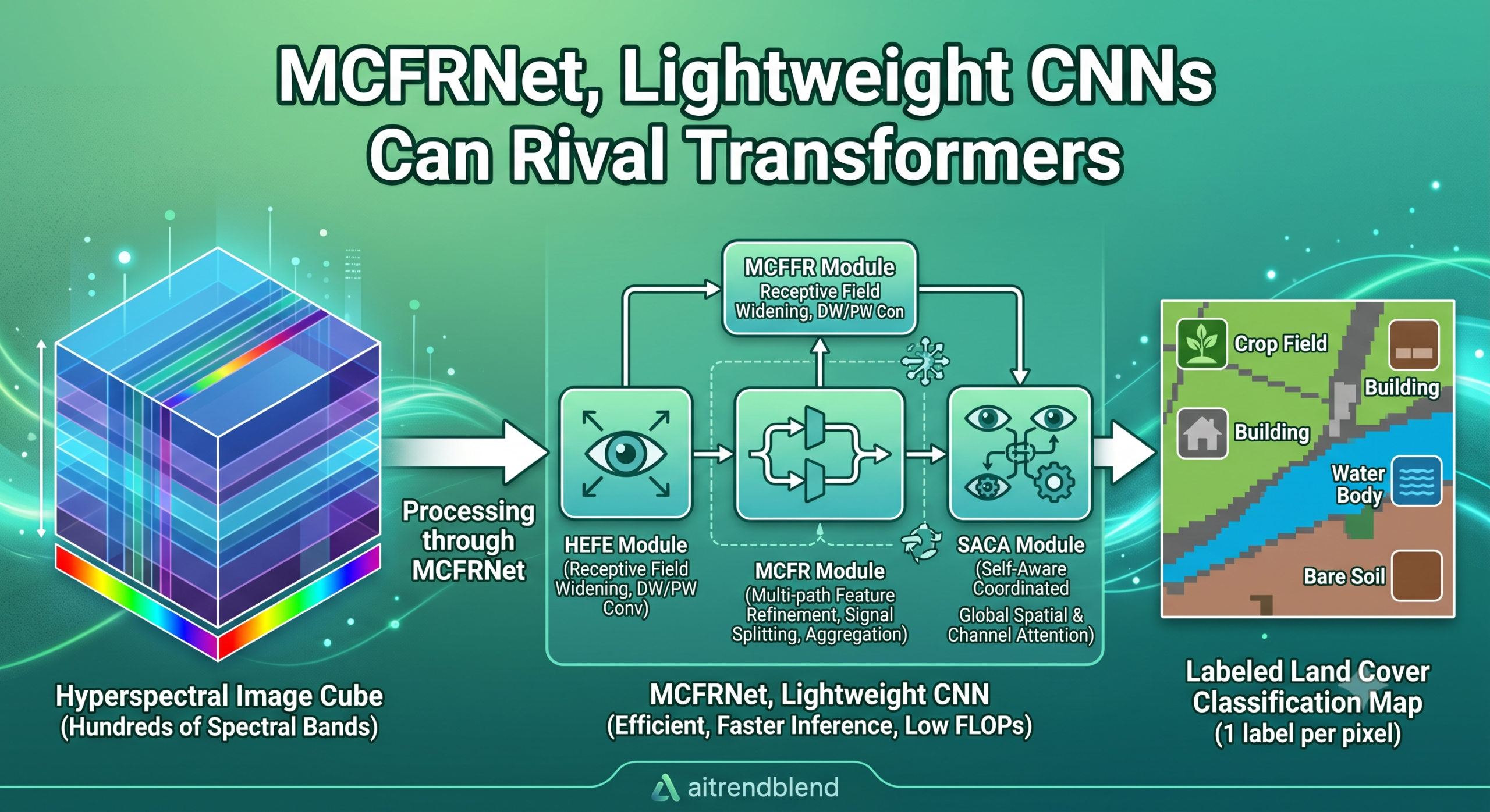
- MCFRNet is a lightweight network built from three modules, each targeting a different part of the tradeoff between contextual reach, fine detail, and computational cost.
- A module called HEFE widens the effective receptive field using depthwise and pointwise convolution instead of expensive standard convolution or self attention.
- A second module, MCFR, separately reconstructs strong and weak feature responses and aggregates information across grouped channel subspaces before recombining them.
- A third module, SACA, combines channel attention with a compact form of global spatial attention to sharpen which spectral bands and spatial regions matter most.
- Across four public hyperspectral benchmarks, MCFRNet posts the best overall accuracy while also running with the fewest FLOPs and the fastest inference time among ten compared methods.
The tradeoff nobody has fully escaped
Hyperspectral images are not ordinary photographs. Where a standard camera captures three color channels, a hyperspectral sensor captures hundreds of narrow, adjacent spectral bands per pixel, turning every single pixel into a rich chemical fingerprint of whatever material it is looking at. That density of information is exactly why hyperspectral imaging shows up in agricultural monitoring, mineral exploration, and environmental surveying, distinguishing between two visually identical patches of ground often comes down to subtle differences buried in that spectral signature rather than anything a human eye could see.
Classifying that data well means solving two problems at once. A network needs a wide enough field of view to understand context, whether a pixel sits inside a large uniform field of one crop or near a boundary where several land types meet. At the same time, it needs to preserve fine, pixel level detail, because the boundaries between spectrally similar categories are exactly where classifiers tend to fail. Convolutional networks are naturally good at the second half of that problem and naturally weak at the first, since a convolution only ever looks at its local neighborhood. Transformer based methods flip that weakness around, self attention can relate any pixel to any other pixel regardless of distance, but that same mechanism is computationally expensive and, in the authors’ assessment, tends to blur exactly the fine local boundaries a convolution would have preserved.
Why the usual fixes only address half the problem
The paper walks through how the field arrived at this impasse. Early hyperspectral classification leaned on classical machine learning, support vector machines, Bayesian estimation, and random forests, often paired with dimensionality reduction techniques like principal component analysis to tame the sheer number of spectral bands. Those methods work reasonably well but struggle once the spatial distribution gets complex or the spectral differences between classes get subtle, their hand crafted features simply were not built to capture that kind of nuance.
Deep learning changed that by letting networks learn their own hierarchical features directly from the data. Three dimensional convolutional networks, which process the spectral and spatial dimensions of a hyperspectral cube jointly, became a natural fit and produced steady improvements, methods like the spectral spatial residual network and the fast dense spectral spatial convolution model pushed accuracy higher by going deeper or adding residual connections. But depth and parameter count both work against a field where labeled training data is chronically scarce, and every added layer raises the risk of overfitting to a small labeled set.
Attention mechanisms entered next, letting networks assign adaptive importance to specific channels or spatial regions rather than treating every input equally. Methods like the dual attention network and RSSAN improved feature recalibration meaningfully, but the authors note a persistent limitation, these attention mechanisms were still bolted onto fundamentally local convolutional backbones, so the underlying receptive field problem never actually went away.
Transformer based approaches arrived as the most direct attack on that receptive field problem, tokenizing hyperspectral patches and applying self attention to model relationships across the entire input. Methods like SpectralFormer, LESSFormer, and GAHT genuinely capture long range dependencies that pure convolution cannot reach. The tradeoff, as the authors frame it, is that tokenization and full self attention introduce real computational overhead and can wash out the sharp local boundaries that convolutional inductive bias naturally protects, which matters enormously when the classes you are trying to separate look spectrally almost identical.
Three modules, three different jobs
Rather than picking a side, MCFRNet is organized as a single pipeline where each stage handles one specific part of the problem, widening context first, then refining what that wider context actually produced, then recalibrating the result adaptively. It helps to walk through the pipeline in the order data actually flows through it.
HEFE, widening the view without the usual cost
Before any of the refinement modules can do their job, the network needs a broader effective receptive field than a plain convolution provides. The High Efficiency Feature Extraction module, HEFE, does this using depthwise convolution followed by two pointwise convolutions, an approach borrowed from efficient mobile architectures rather than from self attention. A residual connection preserves the original spectral spatial information extracted by the initial three dimensional convolution, and an anti bottleneck design temporarily expands the channel dimension to four times its input size between the two pointwise layers, which the authors argue lets the module fully absorb the spatial information the depthwise convolution just extracted before compressing back down. Every convolution in this module is followed by ReLU6 and batch normalization. The authors are explicit that HEFE is not meant to be a universal replacement for standard convolution, it is a lightweight, purpose built front end whose only job is handing a wider effective context downstream without inflating the parameter count.
MCFR, deciding what to trust and what to reuse
Widening the receptive field is not free of side effects. Once HEFE has broadened the context each pixel draws on, the resulting feature responses inevitably include some genuinely useful signal mixed with redundant or unreliable activations, a natural consequence of high spectral redundancy, classes that look spectrally similar, and a training set with very few labeled examples per class. The Multi-path Contextual Feature Refinement module, MCFR, is built specifically to clean this up, and it does so through two complementary mechanisms rather than one.
Multi-layer feature reconstruction separates strong signal from weak signal
The first mechanism, multi-layer feature reconstruction, computes an adaptive, per channel threshold from the feature map itself, then splits every response into a strong component sitting above that threshold and a weak component sitting below it. The strong responses, which likely correspond to genuinely discriminative activations, get passed through a straightforward convolution that preserves their detail. The weak responses get run through a depthwise convolution followed by a softmax, a comparatively cheap operation meant to extract whatever residual semantic value those weaker activations still hold rather than discarding them outright. The two reconstructed streams are then added back together, so the network keeps benefiting from strong signal while still squeezing some use out of the weaker one instead of throwing it away.
Multi-group contextual feature aggregation weighs entire subspaces
The second mechanism, multi-group contextual feature aggregation, works at a coarser level than individual activations. It splits the feature map into several channel groups, treating each group as its own spectral spatial subspace, then learns a softmax based attention mask per group and applies it before all the groups get concatenated back together. Where the first mechanism decides which individual activations to trust, this one decides how much each entire subspace of channels should contribute to the final representation. The authors describe the two as genuinely complementary rather than redundant, one operates on activation strength, the other on group level contextual importance, and a small amount of lightweight local attention, using pooled horizontal and vertical descriptors, is layered on afterward to sharpen spatial structure in the combined result.
SACA, the final adaptive recalibration
The last stage, Self-Aware Coordinated Attention, SACA, takes the refined output from MCFR and applies two more attention mechanisms in tandem. A channel attention branch pools information globally, using both average and max pooling, to figure out which spectral channels carry the most useful information for the task at hand. In parallel, a global spatial attention branch, built from query, key, and value projections in the same spirit as self attention, models long range spatial correlations within the input patch. The two branches are fused multiplicatively rather than just being summed, which the authors describe as a coordinated gating strategy, letting the spatial attention branch’s output be selectively strengthened specifically where the channel attention branch says the spectral information is worth trusting.
It is worth noting exactly why SACA’s self attention style branch stays cheap where a full transformer’s would not. Because the network operates on small, fixed size local patches, typically eleven by eleven or fifteen by fifteen pixels, and because the query and key projections are mapped down to a reduced channel dimension rather than the network’s full channel width, the spatial attention matrix here stays small and manageable rather than scaling up to the size a full image transformer would require.
Does it actually perform, across four genuinely different landscapes
The authors test MCFRNet on four public benchmarks that differ meaningfully in scale, sensor, and land cover type, Houston2013, an urban scene captured over Houston with fifteen distinct ground classes, Pavia University, an academic urban area in northern Italy with nine classes, and two agricultural datasets from Hubei Province in China, WHU-Hi-HanChuan and WHU-Hi-LongKou, both far larger in pixel count and dominated by crop categories that can look spectrally very close to one another. Every method is trained on just one percent of the labeled samples per dataset, a deliberately harsh, low label regime meant to mimic how little annotated hyperspectral data is typically available in practice.
Against nine competing methods, spanning a mix of established CNN, hybrid, and transformer based architectures published between 2022 and 2025, MCFRNet posts the best overall accuracy on every single one of the four datasets. The margin varies a lot depending on how difficult the dataset is. On Houston2013, arguably the hardest of the four because of its fragmented urban structures and strong spectral confusion between categories, MCFRNet improves overall accuracy by a full 1.2 percentage points over the next best method. On Pavia University and the two WHU-Hi agricultural datasets, where several recent methods already sit close to a ceiling in the high nineties, the margin shrinks to somewhere between 0.17 and 0.48 percentage points, which the authors are upfront about, describing it as a ceiling effect rather than a weakness of their own method.
| Dataset | Best competing method | Best competing OA | MCFRNet OA |
|---|---|---|---|
| Houston2013 | MASSFormer | 90.04% | 91.24% |
| Pavia University | MCTGCL | 97.67% | 98.20% |
| WHU-Hi-HanChuan | SYNet | 96.82% | 97.03% |
| WHU-Hi-LongKou | SYNet | 99.48% | 99.65% |
Just as important as the headline accuracy number is where MCFRNet does not win. The authors are candid that their method does not top every single individual category on every dataset, for example, on Houston2013 competing methods classify the Trees, Road, Highway, Railway, and one of the Parking Lot categories more accurately, and on Pavia University, Asphalt, Meadows, Bricks, and Shadows each get classified better by one competitor or another. The advantage, in the authors’ own framing, sits in the overall balance across all categories rather than uniform dominance in every individual class, a distinction worth taking seriously rather than glossing over.
Checking whether the accuracy comes cheap or comes at a real cost
A model that wins on accuracy but demands enormous compute is a much less interesting result for a field where hyperspectral sensors are frequently deployed on resource constrained platforms like drones and satellites. This is where MCFRNet’s numbers get more decisively convincing. Measured on the same hardware across all four datasets, MCFRNet posts both the lowest computational cost and the fastest inference time among all ten compared methods, requiring just over twelve million FLOPs on three of the four datasets and under twenty five million on the largest, versus well over two hundred million FLOPs for some of the more elaborate transformer based competitors. Inference time tells the same story even more starkly, MCFRNet finishes classifying the entire WHU-Hi-HanChuan test set in under a minute, where several competing methods take between three and six times as long on identical hardware.
Parameter count is the one place MCFRNet does not claim outright superiority, sitting in the middle of the pack at roughly one hundred thirty thousand parameters, more than the leanest competitors but comfortably below several of the larger hybrid and transformer architectures. The authors frame this honestly as a tradeoff rather than a clean win across every efficiency axis, prioritizing FLOPs and inference speed, which matter more directly for real time or resource constrained deployment, over squeezing the absolute smallest parameter count.
What the ablation experiments actually establish
A three module architecture invites an obvious question, does each piece genuinely earn its place, or is the accuracy gain really coming from just adding more parameters somewhere. The paper answers this two separate ways, and both are worth taking seriously.
The first is a component ablation, starting from HEFE alone and adding MFR, MCFA, and SACA one at a time. Every addition improves overall accuracy on every dataset, and the improvements are consistent rather than concentrated in just one setting. Removing HEFE entirely, replacing it with nothing while keeping MCFR and SACA in place, causes a measurable performance drop, confirming that HEFE’s job of widening the effective receptive field genuinely matters to what the later modules have to work with. The full combination of all three modules beats every partial combination on every dataset tested.
The second, arguably more convincing check is a replacement based ablation, where each module is swapped for a reasonable alternative rather than simply removed. HEFE is replaced by a standard convolution block and separately by a parameter matched depthwise separable convolution block. MCFR is replaced by simple addition based fusion and by concatenation based fusion. SACA is replaced by plain channel attention and by the widely used convolutional block attention module. In every one of these six substitutions, the full MCFRNet configuration wins on accuracy, which is a stronger claim than the component ablation alone, since it shows each module is not just useful compared to having nothing there but genuinely more effective than a reasonable, comparably sized alternative doing a similar job.
Generalizing beyond a single scene
Accuracy on one labeled scene does not guarantee a model handles a genuinely new scene well, so the authors run a cross scene test using two paired datasets, Houston2013 alongside Houston2018, and Pavia University alongside Pavia Center. MCFRNet posts the highest overall accuracy and average accuracy on all four scenes tested while also requiring the least inference time in every case, evidence that the efficiency gains are not coming at the expense of adaptability to a different capture of a similar environment. This matters practically, since a model destined for real deployment rarely gets evaluated on the exact same scene it was trained on forever.
Honest limitations worth keeping in mind
The authors devote real space to where MCFRNet still falls short rather than only celebrating the headline numbers. On Houston2013 specifically, several individual categories, road, highway, and one parking lot type among them, classify meaningfully worse than the overall average, which the authors attribute to genuinely dispersed, fragmented land cover patterns and high spectral similarity between certain building and vegetation types that a purely spectral spatial approach struggles to fully disentangle. On the datasets where recent competing methods already sit close to a saturation point in the high nineties, MCFRNet’s margin of improvement shrinks to a fraction of a percentage point, which the authors describe candidly as a ceiling effect rather than evidence of a uniquely powerful architecture. The parameter count, while moderate, is not the smallest among compared methods, so a deployment scenario that specifically prioritizes minimal model size over inference speed might still prefer a leaner alternative. Finally, the authors flag their own next research direction directly, incorporating morphological and frequency domain feature extraction to better separate the spectrally similar vegetation and building categories that currently cause the most confusion.
Conclusion
The core contribution here is a genuinely coordinated three module pipeline rather than a single clever trick. HEFE widens the effective receptive field cheaply, MCFR cleans up what that wider context actually produced by separately handling response reliability and group level contextual consistency, and SACA applies one final adaptive pass that decides which spectral channels and spatial regions the refined representation should actually trust. Each module is shown, through both a straightforward ablation and a more demanding replacement based ablation, to be doing real work rather than just adding harmless extra parameters.
The more interesting conceptual takeaway is what this design implies about the CNN versus transformer debate in hyperspectral classification specifically. Rather than treating broader context and computational efficiency as an unavoidable tradeoff, the paper’s central bet is that carefully placed, purpose built modules, none of them a full transformer block, can recover most of the benefit of long range modeling without paying the computational or local detail cost that comes with genuine self attention over an entire input. The efficiency numbers, the lowest FLOPs and fastest inference time among ten compared methods, are the clearest evidence that bet paid off in this setting.
Whether this specific three module recipe transfers cleanly to other dense, high dimensional imaging domains beyond hyperspectral remote sensing, medical volumetric imaging or multispectral agricultural drone footage, for instance, is an open question the paper does not attempt to answer, and the reduced channel query key projection trick that keeps SACA cheap specifically depends on operating over small, fixed size patches rather than full images.
The remaining gaps, uneven performance on a handful of spectrally confusing categories, a shrinking margin on datasets where the field has already nearly saturated accuracy, and a parameter count that is moderate rather than minimal, mark reasonable next steps rather than undermining the central result. The authors themselves point toward morphological and frequency domain features as their next avenue of investigation.
What is worth carrying away from this paper is the reminder that beating a transformer on accuracy is not actually the hardest part of this problem anymore. Beating it on accuracy, inference speed, and computational cost all at once, on four genuinely different real world scenes, is the more demanding bar, and it is the bar this particular architecture was deliberately built to clear.
A runnable implementation of the HEFE, MCFR, and SACA modules
The following is a simplified but complete and runnable reimplementation of the paper’s three core modules, following the equations and design described in Sections 2.2 through 2.4, along with a smoke test that runs a small hyperspectral patch through the full pipeline end to end.
import torch.nn as nn
import torch.nn.functional as F
# —————————————————————–
# HEFE, High Efficiency Feature Extraction, following Eq. 2 to Eq. 4
# Depthwise convolution widens the receptive field, two pointwise
# convolutions with an anti bottleneck expansion integrate channels
# —————————————————————–
class HEFE(nn.Module):
def __init__(self, channels, kernel_size=3, expansion=4):
super().__init__()
padding = kernel_size // 2
self.dwconv = nn.Conv2d(channels, channels, kernel_size, padding=padding, groups=channels)
self.bn_d = nn.BatchNorm2d(channels)
hidden = channels * expansion
self.pwconv1 = nn.Conv2d(channels, hidden, kernel_size=1)
self.bn_e = nn.BatchNorm2d(hidden)
self.pwconv2 = nn.Conv2d(hidden, channels, kernel_size=1)
self.bn_h = nn.BatchNorm2d(channels)
def forward(self, x_3d):
# Eq. 2, depthwise conv plus residual, then ReLU6 and batch norm
f_d = self.bn_d(F.relu6(self.dwconv(x_3d)) + x_3d)
# Eq. 3, expand to four times the channel width
f_e = self.bn_e(F.relu6(self.pwconv1(f_d)))
# Eq. 4, project back down to the original channel width
f_h = self.bn_h(F.relu6(self.pwconv2(f_e)))
return f_h
# —————————————————————–
# MFR, Multi-layer Feature Reconstruction, following Eq. 12 to Eq. 20
# Splits activations into strong and weak components using an
# adaptive per channel threshold, then reconstructs each separately
# —————————————————————–
class MFR(nn.Module):
def __init__(self, channels):
super().__init__()
self.pool = nn.AdaptiveAvgPool2d(1)
self.conv_w1 = nn.Conv2d(channels, channels, kernel_size=1)
self.conv_w2 = nn.Conv2d(channels, channels, kernel_size=1)
self.bn_w1 = nn.BatchNorm2d(channels)
self.bn_w2 = nn.BatchNorm2d(channels)
self.conv_up = nn.Conv2d(channels, channels, kernel_size=1)
self.dwconv_low = nn.Conv2d(channels, channels, kernel_size=3, padding=1, groups=channels)
self.conv_low = nn.Conv2d(channels, channels, kernel_size=1)
self.conv_recal = nn.Conv2d(channels, channels, kernel_size=1)
def forward(self, f_g):
# Eq. 12, adaptive per channel threshold
threshold = torch.sigmoid(self.pool(f_g))
# Eq. 13, two independent response maps
w1 = torch.sigmoid(self.bn_w1(self.conv_w1(f_g)))
w2 = F.relu(self.bn_w2(self.conv_w2(f_g)))
# Eq. 14 and Eq. 15, strong and weak masks via threshold comparison
strong_mask_1 = (w1 >= threshold).float()
weak_mask_1 = (w1 < threshold).float()
strong_mask_2 = (w2 >= threshold).float()
weak_mask_2 = (w2 < threshold).float()
# Eq. 16 and Eq. 17, reconstruct strong and weak responses
p_up = (w1 * strong_mask_1) * f_g + (w2 * strong_mask_2) * f_g
p_low = (w1 * weak_mask_1) * f_g + (w2 * weak_mask_2) * f_g
# Eq. 18, preserve strong response detail with a plain 1×1 conv
p_new_up = self.conv_up(p_up)
# Eq. 19, extract residual semantic value from weak responses cheaply
p_new_low = F.softmax(self.conv_low(self.dwconv_low(p_low)), dim=1)
# Eq. 20, combine reconstructed strong and weak features
p_n = p_new_up + p_new_low
# Eq. 21, a separate channel recalibration branch to suppress noise
p_m = torch.sigmoid(self.conv_recal(self.pool(f_g))) * f_g
return p_n, p_m
# —————————————————————–
# MCFA, Multi-group Contextual Feature Aggregation, following Eq. 8 to Eq. 11
# Splits channels into groups, learns a per group attention mask, and
# recombines the reweighted groups
# —————————————————————–
class MCFA(nn.Module):
def __init__(self, channels, num_groups=4):
super().__init__()
assert channels % num_groups == 0
self.num_groups = num_groups
group_dim = channels // num_groups
self.group_convs = nn.ModuleList([
nn.Conv2d(group_dim, group_dim, kernel_size=1) for _ in range(num_groups)
])
def forward(self, f_g):
# Eq. 8, split along the channel dimension into equal groups
groups = torch.chunk(f_g, self.num_groups, dim=1)
refined_groups = []
for group, conv in zip(groups, self.group_convs):
# Eq. 9, group wise attention mask via softmax over channels
mask = F.softmax(conv(group), dim=1)
# Eq. 10, apply the mask to its own group
refined_groups.append(mask * group)
# Eq. 11, concatenate the refined groups back together
return torch.cat(refined_groups, dim=1)
# —————————————————————–
# SACA, Self-Aware Coordinated Attention, following Eq. 28 to Eq. 41
# Channel attention plus a compact global spatial attention branch,
# fused multiplicatively rather than by simple addition
# —————————————————————–
class SACA(nn.Module):
def __init__(self, channels, reduced_dim=None):
super().__init__()
reduced_dim = reduced_dim or max(channels // 4, 8)
# channel attention branch, Eq. 28 to Eq. 33
self.shared_conv1 = nn.Conv2d(channels, reduced_dim, kernel_size=1)
self.shared_conv2 = nn.Conv2d(reduced_dim, channels, kernel_size=1)
# global spatial attention branch, Eq. 34 to Eq. 38
self.query_conv = nn.Conv2d(channels, reduced_dim, kernel_size=1)
self.key_conv = nn.Conv2d(channels, reduced_dim, kernel_size=1)
self.value_conv = nn.Conv2d(channels, channels, kernel_size=1)
self.reduced_dim = reduced_dim
def forward(self, y):
n, c, h, w = y.shape
# Eq. 28, 29, channel descriptors via average and max pooling
f_avg = F.adaptive_avg_pool2d(y, 1)
f_max = F.adaptive_max_pool2d(y, 1)
# Eq. 30, 31, shared 1×1 convs map both descriptors
m_avg = self.shared_conv2(F.relu(self.shared_conv1(f_avg)))
m_max = self.shared_conv2(F.relu(self.shared_conv1(f_max)))
# Eq. 32, 33, channel attention map and channel enhanced feature
m_ca = torch.sigmoid(m_avg + m_max)
x_ca = y * m_ca
# Eq. 34 to 36, query key value projections over a compact patch
q = self.query_conv(y).view(n, self.reduced_dim, h * w)
k = self.key_conv(y).view(n, self.reduced_dim, h * w)
v = self.value_conv(y).view(n, c, h * w)
# Eq. 37, spatial attention normalized along the token dimension
attn = F.softmax(torch.bmm(q.transpose(1, 2), k) / (self.reduced_dim ** 0.5), dim=-1)
# Eq. 38, spatially enhanced feature reshaped back to a feature map
o = torch.bmm(v, attn.transpose(1, 2)).view(n, c, h, w)
# Eq. 39, residual connection for the spatially enhanced feature
x_gsa = o + y
# Eq. 40, 41, multiplicative fusion of channel and spatial branches
x_1 = x_gsa * x_ca
return x_1 + x_gsa
# —————————————————————–
# The full MCFRNet pipeline wiring HEFE, MCFR (MFR plus MCFA), and SACA
# together, followed by a classification head
# —————————————————————–
class MCFRNet(nn.Module):
def __init__(self, in_channels, num_classes, base_channels=64, num_groups=4):
super().__init__()
self.stem = nn.Conv2d(in_channels, base_channels, kernel_size=3, padding=1)
self.hefe = HEFE(base_channels)
self.split_s = nn.Conv2d(base_channels, base_channels, kernel_size=1)
self.split_r = nn.Conv2d(base_channels, base_channels, kernel_size=1)
self.mfr = MFR(base_channels)
self.mcfa = MCFA(base_channels, num_groups=num_groups)
self.saca = SACA(base_channels)
self.pool = nn.AdaptiveAvgPool2d(1)
self.dropout = nn.Dropout(0.3)
self.fc = nn.Linear(base_channels, num_classes)
def forward(self, x):
# x, shape (batch, in_channels, height, width), a PCA reduced hyperspectral patch
f_3d = self.stem(x)
f_h = self.hefe(f_3d)
# Eq. 5 to 7, align and fuse two branches before MCFR
f_s = torch.sigmoid(self.split_s(f_h))
f_r = F.relu(self.split_r(f_h))
f_g = f_s + f_r
p_n, p_m = self.mfr(f_g)
p_z = self.mcfa(f_g)
# Eq. 22, aggregate the reconstruction, recalibration, and MCFA branches
p = p_m + p_n + p_z
y = self.saca(p)
pooled = self.pool(y).flatten(1)
return self.fc(self.dropout(pooled))
# —————————————————————–
# Smoke test, a small batch of synthetic PCA reduced hyperspectral
# patches trained for a few steps to confirm the pipeline runs
# —————————————————————–
def run_smoke_test():
torch.manual_seed(0)
batch, in_channels, patch_size, num_classes = 8, 30, 11, 15
model = MCFRNet(in_channels, num_classes, base_channels=32)
optimizer = torch.optim.Adam(model.parameters(), lr=0.0003)
loss_fn = nn.CrossEntropyLoss()
for step in range(10):
patches = torch.randn(batch, in_channels, patch_size, patch_size)
labels = torch.randint(0, num_classes, (batch,))
optimizer.zero_grad()
logits = model(patches)
loss = loss_fn(logits, labels)
loss.backward()
optimizer.step()
if step % 2 == 0:
print(f”step {step}, loss {loss.item():.4f}”)
num_params = sum(p.numel() for p in model.parameters())
print(f”total trainable parameters, {num_params:,}”)
if __name__ == “__main__”:
run_smoke_test()
Running this trains the small network for ten steps on random eleven by eleven synthetic patches, printing the loss as it goes and finally reporting the total parameter count, so you can confirm the full HEFE, MCFR, SACA pipeline runs correctly before swapping in a real, PCA reduced hyperspectral dataset and the full patch extraction pipeline described in the paper.
Go straight to the source
This article summarizes and analyzes the original research. Read the full methodology, all eight result tables across four datasets, the complete ablation studies, and the cross scene experiments directly from the publisher, and check the authors’ own repository for their reference implementation.
Read the paper View the code repositoryFrequently asked questions
Why is hyperspectral image classification harder than ordinary image classification?
Each pixel carries hundreds of spectral measurements instead of just three color channels, which provides richer information about material composition but also introduces high dimensionality, spectral redundancy, and subtle differences between classes that are easy for a model to confuse.
What is the main tradeoff between CNN based and transformer based methods for this task?
Convolutional networks are efficient and preserve fine local detail but their limited receptive field restricts how much surrounding context they can consider. Transformer based methods can model long range dependencies across an entire input but typically cost more to compute and can weaken the fine local boundaries that distinguish spectrally similar classes.
What do the three modules in MCFRNet actually do?
HEFE cheaply widens the effective receptive field using depthwise and pointwise convolution. MCFR then refines the resulting features by separately reconstructing strong and weak activations and aggregating information across grouped channel subspaces. SACA applies a final adaptive pass combining channel attention with a compact form of global spatial attention.
Does MCFRNet outperform every competing method on every single land cover category?
No, and the authors are direct about this. It achieves the best overall accuracy on all four datasets tested, but several individual categories on each dataset are still classified more accurately by one competing method or another, meaning its advantage lies in the overall balance rather than uniform dominance everywhere.
How efficient is MCFRNet compared to the methods it was tested against?
Very efficient by the paper’s own measurements. Among ten compared methods, it posts both the lowest computational cost, measured in FLOPs, and the fastest inference time on every one of the four benchmark datasets, while its parameter count sits in the middle of the field rather than being the smallest.
Has this method been tested on data it was not trained on?
Yes. The paper reports a cross scene experiment using paired datasets from the same city captured under different conditions, and MCFRNet achieves the best accuracy and the fastest inference time across all of the cross scene settings tested.
Academic citation. Wan, X., Sun, Z., He, Y., and Chen, F. MCFRNet, multi-path contextual feature refinement network for hyperspectral image classification. Neural Networks, 205, 109341, 2027.
This analysis is based on the published paper and an independent evaluation of its claims.