
Key points
- The model trains its own cerebrospinal fluid segmentation network using labels generated by an existing, imperfect brain imaging tool rather than expensive expert annotations.
- A new feature extraction step measures fluid volume separately across ten slices of brain depth instead of collapsing it into one overall number, and this local detail is what drives most of the accuracy gain.
- On a set of 105 confirmed NPH patients and 112 non-NPH patients, the full system reached 88 percent accuracy, 97 percent sensitivity, and 79 percent specificity.
- Head to head against neuroradiologists reading the same scans by eye, the model matched or beat them on accuracy and sensitivity, including on borderline cases where the radiologists could not reach a confident call at all.
- Specificity lagged behind the radiologists, meaning the model flags more false positives, a tradeoff the authors made deliberately to avoid missing a treatable condition, and one that matters for how the tool should actually be used in a clinic.
A diagnosis that hinges on a number nobody agrees how to measure
Normal pressure hydrocephalus, usually shortened to NPH, shows up mostly in older adults as a triad of gait impairment, urinary incontinence, and cognitive decline, caused by cerebrospinal fluid building up in the brain’s ventricular system. What makes it clinically important, beyond how common it is in elderly populations, is that it can often be treated with a ventricular shunt that drains the excess fluid, and catching it early enough genuinely can reverse the symptoms. The problem is that gait trouble, memory loss, and incontinence describe a huge slice of geriatric neurology, including Alzheimer’s disease and ordinary aging, so imaging becomes the tiebreaker.
For decades that tiebreaker has relied on simple linear measurements taken from a single brain slice, most commonly the Evans’ index, a ratio comparing the width of the lateral ventricles to the width of the skull. The trouble with linear measures like this is that they depend heavily on exactly which slice gets chosen for the measurement, and the healthy cutoff value itself shifts with age, which introduces variability that has nothing to do with the disease. A newer approach called the Maximum Eccentricity of the Lateral Ventricles improved on this somewhat but still depends on slice selection. The paper argues that full volumetric segmentation of cerebrospinal fluid, tracing the actual fluid boundary across every slice rather than measuring one cross section, is the more reliable gold standard, but it is also far more labor intensive, and expert neuroradiologists capable of doing it well are in short supply almost everywhere, a shortage that is dramatically worse in low and middle income countries.
Why CT instead of MRI
MRI is generally considered the preferred imaging method for NPH workups because it shows soft tissue detail more clearly than CT. But MRI machines are expensive and scarce compared to CT scanners, and that gap widens sharply outside wealthy countries. The paper cites 2022 OECD and World Health Organization figures showing roughly 29 CT machines per million people against about 17 MRI machines per million across OECD countries, already a meaningful gap. In the Philippines the ratio was 1.1 CT machines per million against just 0.3 MRI machines, and in Cambodia it was 1.2 CT machines per million against a mere 0.1 MRI machines, more than a twelvefold difference. Building a reliable NPH screening tool that works from CT rather than MRI is therefore not a compromise made for convenience, it is a deliberate choice to build something that could actually be deployed where the shortage of both imaging equipment and expert readers is most acute.
How Weakly Supervised AI Learns CSF Segmentation on Brain CT Scans
Training a neural network to trace cerebrospinal fluid boundaries normally requires a large set of scans where an expert has manually outlined the fluid pixel by pixel, which is exactly the expensive, slow bottleneck the paper is trying to route around. Existing automated segmentation tools exist, but the authors found they generalize poorly to a new hospital’s scanner settings and patient population, a failure mode they call the cold start problem, since a tool trained on one imaging setup often needs to relearn from scratch on another.
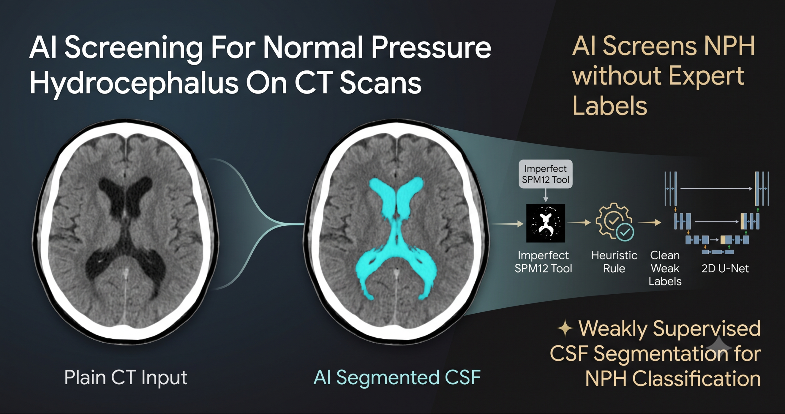
Their solution treats an existing but imperfect brain segmentation tool as a weak labeling function rather than as a final answer. The tool in question is SPM12, an openly available brain imaging toolbox that was never actually designed for precise cerebrospinal fluid extraction on CT scans specifically, and the authors are upfront that its raw output is noisy. Rather than discard those noisy labels, they built a heuristic layer on top of them to clean them up before using them as training targets for a brand new segmentation network.
How the weak labels get built
SPM12 splits each CT slice into four regions, bone, white matter, gray matter, and cerebrospinal fluid, each with a confidence score between zero and one. The team kept only the cerebrospinal fluid pixels where SPM12’s own confidence hit the maximum value of one, treating anything less certain as not fluid at all, a conservative choice that trades some recall for cleaner positive labels. For everything that is not fluid, they used the bone region to trace the interior contour of the skull and subtracted the fluid region from that contour to define a non fluid region. When that contour could not be reliably constructed, which happened more often in slices near the base of the skull, they fell back on the combined white and gray matter regions instead. Everything left over became background.
This process, run across every slice of every training scan, produced a large but noisy set of training examples, three windowed grayscale images per slice paired with a rough CSF versus non CSF versus background mask. Those three grayscale channels come from applying different Hounsfield unit windows to the same CT slice, one tuned to show overall brain structure, one tuned specifically to highlight fluid, and one tuned toward white and gray matter, stacked together as a three channel input image sized down to 224 by 224 pixels.
Training the actual segmentation network
A standard 2D U-Net, four encoder blocks, a bottleneck, and four decoder blocks, was trained on this noisy dataset using a sigmoid focal cross entropy loss, which is a loss function designed to keep training from being dominated by the easy majority class, useful here since background pixels vastly outnumber fluid pixels in a typical brain slice. Training ran for up to two hundred epochs with the Adam optimizer, stopping early if validation loss failed to improve for ten consecutive epochs. The key claim the authors are testing is that a large volume of noisy, heuristically cleaned labels from a tool never designed for this exact task can still produce a better segmentation model than either using that tool’s raw output directly or relying on a model pretrained somewhere else entirely. Their later results suggest that claim holds.
Why the heuristic focuses on just two categories
Reducing the segmentation problem down to fluid versus non fluid, rather than trying to separately identify bone, white matter, and gray matter the way SPM12 does, simplifies what the new network actually has to learn. The authors argue this focus, combined with training on a large number of slices from the actual target hospital’s scanner, let their model outperform the tool that generated its own training labels in the first place.
Turning a fluid mask into features a classifier can use
Once the segmentation model produces a fluid versus non fluid mask for every slice of a brain scan, the next step converts that stack of masks into a fixed length feature vector a simple classifier can work with. The paper defines two core ratios per mask, the CSF ratio, which is fluid pixels divided by fluid plus non fluid pixels, and CSF relative to non CSF, which is fluid pixels divided by non fluid pixels alone.
What makes the feature extraction genuinely interesting is that these two ratios get computed at multiple levels of granularity rather than just once for the whole brain. The global level simply sums fluid and non fluid pixels across the entire scan, producing the kind of single overall volume number that most prior NPH classification work has relied on. The local level instead slices the brain into ten equal partitions along the axial axis, roughly top to bottom, and computes the same two ratios separately within each partition, plus four statistical summaries, minimum, mean, maximum, and standard deviation, calculated from the individual per slice ratios within each partition. That combination produces 104 total features, 20 from the per partition calculations, 80 from the per slice statistical summaries, and 4 from the simple global totals.
The reasoning behind this local breakdown is grounded in something neuroradiologists already look for, that cerebrospinal fluid does not accumulate uniformly across NPH patients, certain brain depths show disproportionate enlargement compared to others. A single whole brain fluid volume number averages that pattern away entirely. Since 104 features is a lot relative to a dataset of only a couple hundred patients, the authors ran a feature selection step using an Extra Trees model to rank feature importance, then tested keeping the top 10, 20, 50, or 100 features against using all of them, ultimately settling on the top 10 features as the best tradeoff between classification performance and model complexity, confirmed through a broader hyperparameter search across different partition counts documented in the paper’s appendix.
What the results actually show
The evaluation used 217 patients, 105 confirmed NPH cases and 112 non-NPH controls, split into a stratified 5 fold cross validation, with an additional pool of 227 NPH patients folded into each training split to add variety without touching the held out test data. The final classifier, a LightGBM model trained on the ten selected local and global features, reached an accuracy of 0.88, a sensitivity of 0.97, a specificity of 0.79, an F1 score of 0.89, and an area under the ROC curve in the low to mid 0.90s depending on which table in the paper you read, with the abstract reporting 0.91 and the main results table reporting 0.93 for this exact configuration.
| Segmentation source | Feature type | Accuracy | Sensitivity | Specificity |
|---|---|---|---|---|
| SPM12 direct output | Global only | 0.57 | 0.68 | 0.47 |
| Pretrained 2D U-Net | Global only | 0.68 | 0.70 | 0.66 |
| Weak supervised U-Net (proposed) | Global only | 0.71 | 0.78 | 0.65 |
| Pretrained 3D U-Net | Selected local + global | 0.83 | 0.87 | 0.80 |
| Pretrained 2D U-Net | Selected local + global | 0.86 | 0.93 | 0.79 |
| Weak supervised U-Net (proposed) | Selected local + global | 0.88 | 0.97 | 0.79 |
Two separate effects are worth pulling apart from that table, because they get conflated if you only glance at the headline numbers. Switching from global only features to the full local plus global feature set improved every single segmentation method tested, with F1 score gains reported in the paper ranging from 16 to 32 percent and AU-ROC gains ranging from 15 to 38 percent depending on which underlying segmentation approach was used. That is a large, consistent effect that has nothing to do with which segmentation model generated the mask in the first place. Separately, switching from any of the other four segmentation approaches to the weak supervised model, while holding the feature extraction method constant, produced a smaller but still meaningful further improvement. Both pieces mattered, and the paper’s ablation style comparison in its results table makes that reasonably clear rather than just reporting one combined number.
A separate, smaller check gives some independent confirmation that the segmentation itself genuinely improved. On six CT scans where a senior neuroradiologist with over twenty years of experience manually traced fluid regions on a single slice each, the weak supervised model’s predicted mask reached a mean Dice coefficient of 0.747 against that expert tracing, compared to 0.657 for SPM12’s raw output on the same slices, despite the new model having been trained entirely on SPM12 derived labels to begin with. That is a genuinely notable result, a student model trained on a noisy teacher’s labels ending up more accurate than the teacher itself on an independent expert benchmark, though it is worth flagging that this comparison used only six scans and a single annotated slice per scan, a small sample for a segmentation accuracy claim.
How it stacks up against neuroradiologists
The most clinically relevant comparison in the paper pits the model directly against a panel of two senior neuroradiologists, one with over twenty years of experience and one with over ten, plus a third year radiology resident, who scored the same 217 scans by eye using seven established radiological signs converted into a composite scale called the Radscale, ranging from zero to twelve points. Patients scoring below three were called non-NPH, patients scoring five or above were called NPH, and this group of confident calls covered 87 NPH patients and 93 non-NPH patients. A separate group of 37 patients fell into the middle, a borderline zone where the radiologists’ own scoring system does not produce a confident answer either way.
| Group | Evaluator | Accuracy | Sensitivity | Specificity | F1 |
|---|---|---|---|---|---|
| Confidence group | Neuroradiologists | 0.84 | 0.74 | 0.99 | 0.84 |
| Confidence group | Model (proposed) | 0.91 | 0.98 | 0.85 | 0.91 |
| Borderline group | Neuroradiologists | no call reached | no call reached | no call reached | no call reached |
| Borderline group | Model (proposed) | 0.73 | 0.94 | 0.53 | 0.77 |
On the confidence group, the model beat the radiologists on overall accuracy and sensitivity by a wide margin, catching 98 percent of true NPH cases against the radiologists’ 74 percent, though the radiologists were notably more specific, correctly ruling out 99 percent of non-NPH cases against the model’s 85 percent. On the borderline group, where the radiologists’ own scoring scale could not produce a definitive answer at all, the model still managed a sensitivity of 0.94, which the authors frame as evidence the tool could genuinely help flag at risk patients in exactly the scenario where visual scoring runs out of confidence.
Why the model misses on specificity, and what that means
The authors do not gloss over the specificity gap, and their error analysis digs into it directly. Some non-NPH patients in this dataset have genuinely enlarged ventricles without the clinical symptoms that would justify an NPH diagnosis, and since ground truth labels here were built from a combination of a cerebrospinal fluid tap test, imaging, and clinical presentation, while the model only ever sees the imaging, it has no way to know when a patient’s large ventricles are an incidental finding rather than a symptomatic one. That mismatch between what the model can observe and what actually defines a positive label is a real, structural limitation, not a bug that more training data would obviously fix.
The team also deliberately tuned their model selection to favor lower false negatives over lower false positives, on the reasoning that missing a treatable condition is a worse outcome in a screening context than flagging a patient for a second look who turns out not to have NPH. That is a defensible design choice for a screening tool meant to sit upstream of a full clinical workup rather than to serve as a final diagnosis, but it is a choice, not a neutral default, and it is the direct cause of the lower specificity numbers throughout the results.
A separate investigation checked whether misclassifications were being driven by anatomical misalignment, patients whose brain structures happen to fall into different numbered partitions than most of the training set due to natural anatomical variation. Using SHAP feature importance analysis to trace which features drove individual predictions, the authors found that both correct and incorrect predictions occurred in both aligned and misaligned patients, suggesting the model adapts reasonably well to shifted anatomy as long as the relevant fluid containing partitions are still represented somewhere among its selected features, rather than misalignment alone explaining the error pattern.
Which brain regions actually drove the predictions
The SHAP analysis also identified which of the ten selected features mattered most across the cross validation folds. The majority came from the fifth and sixth partitions, which visual inspection confirmed correspond to the lateral ventricles, the classic anatomical site NPH imaging assessment already focuses on, plus a smaller but consistent contribution from the ninth partition, corresponding to the subarachnoid space near the top of the head. The single most influential feature was the standard deviation of the per slice fluid ratio within that ninth partition, where a low value pushed predictions toward NPH and a high value pushed away from it. That the model’s most important learned features line up with anatomical regions radiologists already know to inspect is a reassuring sign that it is picking up on genuine anatomical signal rather than some spurious artifact of the dataset.
Clinical translation gap
Every result in this paper comes from a single hospital, Siriraj Hospital in Bangkok, using one CT scanner protocol and one patient population. The authors are explicit that this limits how confidently the results generalize to a different hospital with different scanning parameters, and they note this as a limitation they intend to address with future multi hospital validation rather than something already resolved. The weak label generation process itself depends entirely on one external tool, SPM12, and the paper flags that relying on a single labeling source is itself a constraint worth revisiting. There has also been no prospective evaluation, meaning the model has not yet been tested on new patients as they arrive in a real clinical workflow, only retrospectively on scans that were already collected and already had a known outcome. A retrospective dataset like this one also cannot include patients who presented with NPH like symptoms but were ultimately never referred for a CSF tap test or confirmed as non-NPH through full workup, which the authors acknowledge is a gap between this dataset and real world clinical presentation.
Honest limitations
The paper’s own discussion section is unusually candid about where the approach falls short, and it is worth walking through those points directly rather than only reporting the headline numbers. The model still cannot reliably separate NPH patients from non-NPH patients who both happen to have enlarged ventricles, even though it does well at distinguishing non-NPH patients whose ventricles are not enlarged in the first place. The authors suggest this may be because local volumetric differences alone do not capture some of the subtler radiological distinctions between these two overlapping groups, and they point toward future end to end deep learning approaches that could potentially learn more complex patterns directly from raw CT data as a possible next step, though that remains speculative rather than demonstrated.
The fixed choice of ten equal partitions, while empirically the best performing option the authors tested, does not account for the brain’s actual anatomical structure, meaning the same physical brain region could land in a slightly different numbered partition across different patients due to ordinary anatomical variation, a problem spatial normalization only partially corrects. The authors lay out three possible directions for future work here, population specific templates tailored to age or other patient characteristics, a separate model that explicitly detects anatomical regions before extracting features, or an attention based architecture that could learn to focus on informative slices without relying on fixed partitions at all, while being upfront that each option adds its own complexity or interpretability cost.
Where this fits and what comes next
Zoom out and the most transferable idea in this paper is not really about hydrocephalus specifically, it is the weak supervision recipe itself, take an existing tool that was never built for your exact task, apply a domain specific heuristic to clean up its output, and use the resulting noisy but abundant labels to train a purpose built model that ends up more accurate than the tool that supervised it. That pattern could plausibly transfer to other conditions where an imperfect general purpose segmentation tool already exists but a precisely tuned model for one specific clinical question does not. The local feature extraction idea, breaking a single global volume metric into per region measurements along an anatomical axis, is the second transferable idea, and the paper’s own ablation results make a strong case that this decomposition, not just the underlying segmentation quality, is doing a large share of the classification work.
Conclusion
The core achievement here is closing the cold start problem for a specific, useful diagnostic task using a training recipe that costs nothing beyond compute time, no radiologist had to sit down and trace cerebrospinal fluid across hundreds of scans before this model could be trained on the target hospital’s own data. The resulting segmentation model turned out to outperform the very tool that generated its training labels, on both downstream classification accuracy and on an independent expert comparison, a genuinely notable outcome for a weak supervision approach.
The conceptual shift worth remembering is that local variation in cerebrospinal fluid volume across brain depth carries real diagnostic signal that a single global volume number throws away, and the magnitude of the improvement from adding local features, consistent across every segmentation method the authors tested, is the paper’s strongest and most broadly applicable finding.
The honest limitations remain significant. Every number in this paper comes from one hospital’s scanner and one patient population, the model’s lower specificity reflects a deliberate but consequential design tradeoff rather than a solved problem, and the model still struggles on precisely the patients where imaging alone is genuinely ambiguous, those with enlarged ventricles but no NPH diagnosis. None of that erases the value of the head to head comparison against working neuroradiologists, particularly the finding that the model produced a confident, reasonably accurate call on borderline patients where the human panel’s own scoring system could not.
The authors are clear that this is a screening aid meant to support, not replace, expert judgment and the broader clinical workup that a real NPH diagnosis requires, including the cerebrospinal fluid tap test that this dataset’s own ground truth labels were partly built from. Future work the authors point toward, multi hospital validation, prospective testing in real clinical workflows, and architectures that adapt to anatomical variation without fixed partitions, would all matter more to a clinic considering this tool than another fraction of a percentage point on accuracy within this single retrospective dataset.
Read the full peer reviewed paper for the complete equations, the appendix hyperparameter search, and the SHAP analysis figures.
Read the paper in Computers in Biology and Medicine Get the SPM12 toolbox used for weak labelsFrequently asked questions
What is normal pressure hydrocephalus and why does it matter that it be caught early
Normal pressure hydrocephalus is a buildup of cerebrospinal fluid in the brain’s ventricles that causes gait problems, urinary incontinence, and cognitive decline, symptoms that closely resemble Alzheimer’s disease and other forms of dementia. It matters because, unlike most causes of these symptoms, NPH can often be treated with a ventricular shunt that drains the excess fluid, and catching it early can reverse the symptoms rather than just slow their progression.
How did the researchers train a segmentation model without manually labeled scans
They used SPM12, an existing brain imaging toolbox not specifically built for CT based fluid extraction, to generate rough segmentation labels, then applied a heuristic function using the skull’s bone contour to clean up those labels into a cerebrospinal fluid versus non fluid distinction. This noisy but large training set was used to train a new U-Net segmentation model from scratch on the target hospital’s own scans.
How accurate is the model at classifying NPH
Using its best configuration, ten selected local and global volumetric features with a LightGBM classifier, the model reached 88 percent accuracy, 97 percent sensitivity, and 79 percent specificity on a set of 105 confirmed NPH patients and 112 non-NPH patients, evaluated with 5 fold cross validation.
Did the model actually outperform neuroradiologists
On patients where the neuroradiologists reached a confident visual diagnosis, the model matched or exceeded them on overall accuracy and was notably more sensitive, though the radiologists were more specific. On a separate group of borderline patients where the radiologists’ own scoring system could not produce a definitive call, the model still achieved 94 percent sensitivity, suggesting a potential role in supporting screening on exactly the cases where visual assessment runs out of confidence.
What are the biggest limitations of this study
All the data comes from a single hospital and a single CT scanner setup, which limits how confidently the results generalize elsewhere. The model also struggles specifically with distinguishing NPH from non-NPH patients who both have enlarged ventricles, and its lower specificity compared to radiologists reflects a deliberate design choice to prioritize catching potential cases over avoiding false alarms, which may or may not be the right tradeoff depending on how the tool is actually deployed in practice.
Is this model available for clinical use
No. This is a research study evaluated retrospectively on data from one hospital, without prospective clinical validation or regulatory clearance. The authors describe it as a potential screening aid to support neuroradiologists, not a replacement for the full clinical workup, including the cerebrospinal fluid tap test, that an actual NPH diagnosis requires.
Explore more in this pillar
Reproducible Python implementation
The block below is an independent, runnable implementation of the paper’s pipeline, including the weak label heuristic, the local and global volumetric feature extraction algorithm, and the classifier stage, using PyTorch for the segmentation network and scikit-learn style gradient boosting for classification. It ends with a smoke test on random dummy data so you can confirm the shapes and feature counts flow correctly before pointing it at real scans.
# nph_screening.py
# Independent reproduction of the weak supervision NPH screening pipeline
# (Supratak et al., Computers in Biology and Medicine, 2025)
# Not official code from the authors. Written for educational reuse.

import numpy as np
import torch
import torch.nn as nn
import torch.nn.functional as F


def build_weak_labels(csf_prob, bone_prob, wm_prob, gm_prob, confidence_threshold=1.0):
    """
    Reproduces the heuristic weak label construction. All inputs are
    numpy arrays of shape (H, W) with values in [0, 1] representing
    SPM12 style confidence maps for CSF, bone, white matter, gray matter.
    Returns an integer mask: 0 = background, 1 = CSF, 2 = non-CSF.
    """
    csf_mask = (csf_prob >= confidence_threshold).astype(np.uint8)

    # Approximate the interior skull contour from the bone probability map
    # by filling the region enclosed by high confidence bone pixels.
    bone_mask = (bone_prob > 0.5).astype(np.uint8)
    interior_contour = _fill_interior(bone_mask)

    contour_available = interior_contour.sum() > 0
    if contour_available:
        non_csf_mask = np.clip(interior_contour - csf_mask, 0, 1)
    else:
        wm_gm_mask = ((wm_prob > 0.5) | (gm_prob > 0.5)).astype(np.uint8)
        non_csf_mask = np.clip(wm_gm_mask - csf_mask, 0, 1)

    weak_label = np.zeros_like(csf_mask, dtype=np.uint8)
    weak_label[non_csf_mask > 0] = 2
    weak_label[csf_mask > 0] = 1
    return weak_label


def _fill_interior(bone_mask):
    # Simplified stand in for morphological contour filling.
    # A real implementation would use a proper flood fill or convex hull.
    filled = bone_mask.copy()
    for row in range(filled.shape[0]):
        cols = np.where(filled[row] > 0)[0]
        if len(cols) > 1:
            filled[row, cols.min():cols.max()] = 1
    return filled


class DoubleConv(nn.Module):
    def __init__(self, in_ch, out_ch):
        super().__init__()
        self.block = nn.Sequential(
            nn.Conv2d(in_ch, out_ch, 3, padding=1), nn.BatchNorm2d(out_ch), nn.ReLU(inplace=True),
            nn.Conv2d(out_ch, out_ch, 3, padding=1), nn.BatchNorm2d(out_ch), nn.ReLU(inplace=True)
        )

    def forward(self, x):
        return self.block(x)


class CSFUNet(nn.Module):
    """2D U-Net matching the paper's four encoder, bottleneck, four decoder design."""
    def __init__(self, in_ch=3, base=32):
        super().__init__()
        self.enc1 = DoubleConv(in_ch, base)
        self.enc2 = DoubleConv(base, base * 2)
        self.enc3 = DoubleConv(base * 2, base * 4)
        self.enc4 = DoubleConv(base * 4, base * 8)
        self.pool = nn.MaxPool2d(2)
        self.bottleneck = DoubleConv(base * 8, base * 16)

        self.up4 = nn.ConvTranspose2d(base * 16, base * 8, 2, stride=2)
        self.dec4 = DoubleConv(base * 16, base * 8)
        self.up3 = nn.ConvTranspose2d(base * 8, base * 4, 2, stride=2)
        self.dec3 = DoubleConv(base * 8, base * 4)
        self.up2 = nn.ConvTranspose2d(base * 4, base * 2, 2, stride=2)
        self.dec2 = DoubleConv(base * 4, base * 2)
        self.up1 = nn.ConvTranspose2d(base * 2, base, 2, stride=2)
        self.dec1 = DoubleConv(base * 2, base)

        self.head = nn.Conv2d(base, 1, kernel_size=1)

    def forward(self, x):
        e1 = self.enc1(x)
        e2 = self.enc2(self.pool(e1))
        e3 = self.enc3(self.pool(e2))
        e4 = self.enc4(self.pool(e3))
        b = self.bottleneck(self.pool(e4))

        d4 = self.dec4(torch.cat([self.up4(b), e4], dim=1))
        d3 = self.dec3(torch.cat([self.up3(d4), e3], dim=1))
        d2 = self.dec2(torch.cat([self.up2(d3), e2], dim=1))
        d1 = self.dec1(torch.cat([self.up1(d2), e1], dim=1))
        return self.head(d1)


def sigmoid_focal_loss(logits, targets, gamma=2.0, alpha=0.25):
    prob = torch.sigmoid(logits)
    ce = F.binary_cross_entropy_with_logits(logits, targets, reduction="none")
    p_t = prob * targets + (1 - prob) * (1 - targets)
    alpha_t = alpha * targets + (1 - alpha) * (1 - targets)
    loss = alpha_t * (1 - p_t) ** gamma * ce
    return loss.mean()


def extract_volumetric_features(csf_masks, non_csf_masks, num_partitions=10):
    """
    csf_masks and non_csf_masks are lists of 2D binary numpy arrays, one
    per axial slice, ordered along the axial axis. Returns a dict with
    per-partition, per-slice, and global features matching the paper's
    104 feature design when num_partitions is 10.
    """
    num_slices = len(csf_masks)
    n_csf_per_slice = np.array([m.sum() for m in csf_masks], dtype=np.float64)
    n_noncsf_per_slice = np.array([m.sum() for m in non_csf_masks], dtype=np.float64)

    eps = 1e-8
    omega_per_slice = n_csf_per_slice / (n_csf_per_slice + n_noncsf_per_slice + eps)
    psi_per_slice = n_csf_per_slice / (n_noncsf_per_slice + eps)

    partition_bounds = np.linspace(0, num_slices, num_partitions + 1).astype(int)

    per_partition_features = []
    per_slice_stat_features = []

    for p in range(num_partitions):
        start, end = partition_bounds[p], partition_bounds[p + 1]
        idx = slice(start, end)

        # Per-partition: sum counts within the partition first, then ratio
        csf_sum = n_csf_per_slice[idx].sum()
        noncsf_sum = n_noncsf_per_slice[idx].sum()
        omega_p = csf_sum / (csf_sum + noncsf_sum + eps)
        psi_p = csf_sum / (noncsf_sum + eps)
        per_partition_features.extend([omega_p, psi_p])

        # Per-slice: aggregate the per-slice ratios with 4 statistics
        omega_slice_vals = omega_per_slice[idx]
        psi_slice_vals = psi_per_slice[idx]
        for vals in [omega_slice_vals, psi_slice_vals]:
            if len(vals) == 0:
                per_slice_stat_features.extend([0.0, 0.0, 0.0, 0.0])
            else:
                per_slice_stat_features.extend([vals.min(), vals.mean(), vals.max(), vals.std()])

    total_csf = n_csf_per_slice.sum()
    total_noncsf = n_noncsf_per_slice.sum()
    global_omega = total_csf / (total_csf + total_noncsf + eps)
    global_psi = total_csf / (total_noncsf + eps)
    global_sum_omega = omega_per_slice.sum()
    global_sum_psi = psi_per_slice.sum()
    global_features = [global_omega, global_psi, global_sum_omega, global_sum_psi]

    all_features = np.array(per_partition_features + per_slice_stat_features + global_features)
    return {
        "features": all_features,
        "n_features": len(all_features),
        "per_partition": np.array(per_partition_features),
        "per_slice_stats": np.array(per_slice_stat_features),
        "global": np.array(global_features),
    }


if __name__ == "__main__":
    # Smoke test on random dummy data, confirms shapes flow end to end
    device = torch.device("cuda" if torch.cuda.is_available() else "cpu")

    # 1. Weak label generation on a single dummy slice
    H, W = 224, 224
    csf_prob = np.random.rand(H, W)
    bone_prob = np.random.rand(H, W)
    wm_prob = np.random.rand(H, W)
    gm_prob = np.random.rand(H, W)
    weak_label = build_weak_labels(csf_prob, bone_prob, wm_prob, gm_prob)
    print("weak label unique values", np.unique(weak_label))

    # 2. Segmentation model forward and loss
    model = CSFUNet(in_ch=3).to(device)
    dummy_images = torch.rand(2, 3, 224, 224).to(device)
    dummy_targets = (torch.rand(2, 1, 224, 224) > 0.8).float().to(device)
    logits = model(dummy_images)
    loss = sigmoid_focal_loss(logits, dummy_targets)
    print("segmentation loss", loss.item())

    optimizer = torch.optim.Adam(model.parameters(), lr=0.001)
    loss.backward()
    optimizer.step()

    # 3. Volumetric feature extraction on a dummy 120 slice scan
    num_slices = 120
    csf_masks = [(np.random.rand(64, 64) > 0.9) for _ in range(num_slices)]
    non_csf_masks = [(np.random.rand(64, 64) > 0.4) for _ in range(num_slices)]
    result = extract_volumetric_features(csf_masks, non_csf_masks, num_partitions=10)
    print("total feature count", result["n_features"])
    print("smoke test complete")
This analysis is based on the published paper and an independent evaluation of its claims.
Your point of view caught my eye and was very interesting. Thanks. I have a question for you.