
This article explains a published computational biology paper. CelloType is a research tool for analyzing tissue images in spatial omics experiments, it is not a diagnostic device and is not used to make decisions about an individual patient’s care. Any clinical application of tools like this would require separate validation, regulatory review, and oversight by qualified professionals.
Key points
- CelloType combines cell segmentation and cell type classification into one transformer based model instead of running them as two separate steps, using a Swin Transformer backbone, a DINO style detection module, and a MaskDINO style segmentation module.
- On the TissueNet benchmark, CelloType with confidence scores reached a mean average precision of 0.56 for cell segmentation, ahead of Cellpose2 at 0.35 and Mesmer at 0.31.
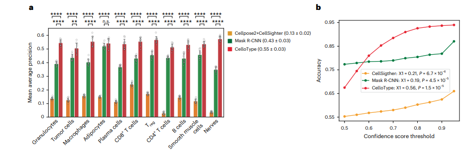
- For joint segmentation and cell type classification on a colorectal cancer CODEX dataset, CelloType reached a mean average precision of 0.55 across cell types, compared with 0.13 for a Cellpose2 plus CellSighter pipeline and 0.43 for Mask R-CNN.
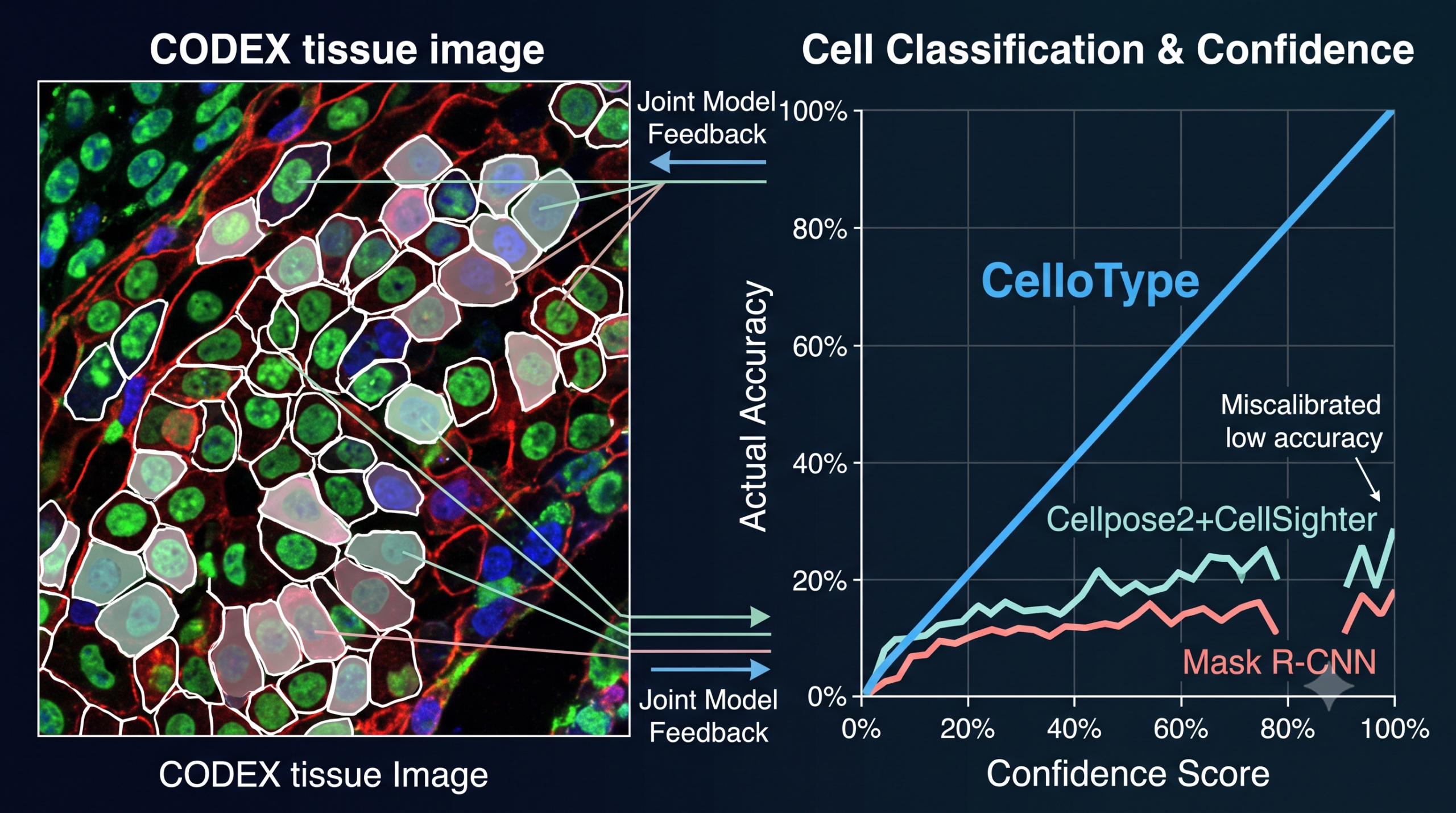
- CelloType’s confidence scores tracked actual prediction accuracy far more closely than the compared methods, with a fitted regression coefficient of 0.56 versus 0.21 and 0.19 for the alternatives.
- That accuracy comes at a real computational cost. The paper’s own extended data show CelloType using roughly three times the training memory and more than double the training time of the two stage baseline it was compared against.
Two jobs that used to be two models
Spatial omics technologies, the family of methods that let researchers image dozens to thousands of molecular markers across an intact piece of tissue, have exploded over the last several years. Consortium efforts like the Human Tumor Atlas Network and the Human Biomolecular Atlas Program are mapping healthy and diseased tissue at cellular resolution, and every one of those maps starts with the same two computational steps. First, find where each cell is, drawing a boundary around it. Second, decide what kind of cell it is, a T cell, a macrophage, a tumor cell, an adipocyte. Conventional pipelines treat these as a strict sequence. Segment first, then feed the resulting masks into a separate classifier. Mesmer, a widely used segmentation tool, pairs a convolutional backbone with a feature pyramid network and a watershed algorithm to draw cell and nuclear boundaries. Cellpose and its successor Cellpose2 take a different route, using a convolutional network to predict a topological gradient map and then tracking that gradient to recover cell shapes. For classification, CellSighter trains a convolutional network to assign cell types using the segmentation masks and the underlying tissue image, while CELESTA takes an iterative approach based on a quantified table of protein expression per cell.
Each of these tools does its one job reasonably well. The problem the CelloType team identified is what gets lost in the handoff between them. A classifier that only sees the final segmentation mask cannot draw on the raw texture and marker intensity patterns that might have helped it recognize a cell type, and a segmentation model trained without any notion of cell type cannot use the fact that, say, macrophages and lymphocytes tend to look different at the pixel level. Training two models separately is also simply more expensive, and the paper notes that segmentation quality itself varies a lot across tissue types and imaging platforms, leaving real room for a method that handles both tasks with shared information.
How CelloType actually works
CelloType’s architecture has three parts, and each one has a specific, traceable job.
A transformer backbone in place of a convolutional one
The first stage extracts multiscale image features using a Swin Transformer, specifically a Swin-L model pretrained on the COCO instance segmentation dataset. Swin Transformer is a hierarchical vision transformer that computes attention within shifted local windows rather than across an entire image at once, which lets it capture both fine local detail and broader spatial context more efficiently than a standard convolutional network. This feature map, called C_b in the paper’s notation, feeds into both of the modules that follow.
DINO for detection, with a query strategy built for crowded cells
The second stage is a DINO module, short for DETR with improved denoising anchor boxes, an object detection architecture built around a transformer encoder and decoder. DINO generates two kinds of query for locating objects. Positional queries are initialized from the encoder’s own top scoring features and represent where an object might be, while content queries are separate learnable embeddings that represent what an object might contain. The paper describes this mixed strategy formally as
where \(X\) represents the flattened image features combined with positional embeddings, \(Q_{pos}\) is an n by 4 matrix of anchor box coordinates, and \(Q_{content}\) is an n by embedding dimension matrix of learnable content vectors.
Decoder layers then refine these anchor boxes using deformable attention, which restricts each query’s attention to a small set of sampling points near its current estimated location rather than scanning the whole image, making the computation considerably cheaper than full attention while still letting boxes adjust as the network learns more about where cells actually are. A contrastive denoising step runs alongside this refinement, deliberately perturbing ground truth boxes by two different noise scales during training.
The paper generates both a positive query with a smaller noise scale, \(\lambda_1 = 0.4\), and a negative query with a larger noise scale, \(\lambda_2 = 1\), teaching the model to recognize a slightly shifted true box while also learning to reject a badly shifted one, which sharpens its ability to tell adjacent or overlapping cells apart.
Once a bounding box settles, a linear layer converts its features into class probabilities, using an ordinary softmax over K classes plus a dedicated no object class so the model can decline to label background regions.
The confidence score reported for each detected cell is simply the highest class probability, excluding the no object class, that the softmax produces for that prediction.
MaskDINO for the actual pixel boundaries
Detection gives boxes, not the precise cell outline a biologist actually wants. That job falls to a MaskDINO style segmentation module, which takes the content query embeddings from the DINO decoder and combines them with the backbone’s image features and the encoder’s latent features to produce a binary mask for every detected instance.
Here \(q_c\) is a content query embedding, \(T\) is a convolutional layer that projects the backbone feature map \(C_b\) into the transformer’s hidden dimension, \(F\) is an upsampling function that brings the encoder’s latent features \(C_e\) up to matching resolution, and \(M\) is the segmentation head that turns the combined map into a per pixel embedding. Each instance mask \(m\) is the dot product between that query’s embedding and the pixel embedding map, essentially asking, at every pixel, how well does this location match the thing this query is describing.
All three modules train together under one composite loss, rather than being optimized in separate stages.
That shared training signal is the mechanical reason CelloType can, in principle, let segmentation and classification inform each other. Object detection features that got better because they help distinguish cell types also feed the mask branch, and a mask branch that gets better at outlining unusual cell shapes changes what the shared encoder learns.
Benchmark by benchmark
TissueNet, the six platform, six tissue type stress test
TissueNet is a substantial multiplexed imaging benchmark, spanning six imaging technologies, CODEX, CycIF, imaging mass cytometry, multiplexed ion beam imaging, multiplexed immunofluorescence, and Vectra, across six tissue types including breast, gastrointestinal, immune, lung, pancreas, and skin. The dataset was split into 2,580 training patches and 1,324 test patches, each 512 by 512 or 256 by 256 pixels.
Using the COCO style average precision metric across intersection over union thresholds from 0.50 to 0.90, CelloType with confidence scoring, labeled CelloType_C in the paper, reached a mean AP of 0.56 for cell segmentation, ahead of the basic CelloType variant at 0.45, Cellpose2 at 0.35, and Mesmer at 0.31. Nuclear segmentation followed the same ordering with a wider gap. CelloType_C scored 0.66, CelloType scored 0.57, Cellpose2 scored 0.52, and Mesmer scored 0.24.
| Method | Cell segmentation mean AP | Nuclear segmentation mean AP |
|---|---|---|
| Mesmer | 0.31 ± 0.01 | 0.24 ± 0.01 |
| Cellpose2 | 0.35 ± 0.02 | 0.52 ± 0.02 |
| CelloType | 0.45 ± 0.02 | 0.57 ± 0.02 |
| CelloType_C | 0.56 ± 0.02 | 0.66 ± 0.02 |
Every method’s performance dropped on imaging mass cytometry data and on breast tissue specifically, a consistent weak spot across the field rather than something unique to any one architecture. The qualitative pattern the authors point to is a useful diagnostic in its own right. Cellpose2 tends to draw boundaries larger than the true cell, undersegmenting and merging what should be separate cells, while Mesmer tends to miss cells and nuclei outright, showing up as a lower recall rate. CelloType’s advantage in the head to head comparisons largely traces back to avoiding both of those specific failure modes rather than to some single dramatic improvement.
Beyond fluorescence, on the Cellpose Cyto dataset
To check whether CelloType’s advantage held up outside multiplexed fluorescence imaging, the team applied it to the Cellpose Cyto dataset, which mixes fluorescence and bright field microscopy images of cells alongside images of ordinary objects like fruit and seashells used as an out of domain stress test for general purpose segmentation. Since Mesmer requires two channel input and most of this dataset is single channel, only Cellpose2 and CelloType were compared here.
CelloType_C reached a mean AP of 0.47 across the full dataset based on ten fold cross validation, ahead of CelloType at 0.37 and Cellpose2 at 0.32, and this ordering held consistently across all six image subsets in the dataset. One detail worth flagging separately concerns training data efficiency. On TissueNet, CelloType’s performance climbed noticeably as more training data was added, reaching a mean AP of only 0.36 with 20 percent of the training set before improving substantially with the full set. On Cellpose Cyto, that sensitivity was much smaller, mean AP moved from 0.44 with 20 percent of the training data to 0.48 with the full amount. The likely explanation is that Cellpose Cyto’s images are visually simpler and more homogeneous than the six platform, six tissue type sprawl of TissueNet, so there is simply less for additional data to teach the model.
Spatial transcriptomics, where transcript signal alone falls flat
Imaging based spatial transcriptomics, which localizes individual RNA transcripts inside tissue rather than relying purely on protein markers, is a fast growing companion technology to spatial proteomics platforms like CODEX. The team tested CelloType on three 10x Genomics Xenium datasets, human lung cancer, pancreas cancer, and mouse normal colon, and on a MERFISH dataset built from human brain tissue with a 4,000 gene panel.
On the Xenium data, CelloType combining DAPI nuclear stain and transcript signal reached a mean AP of 0.47, dramatically ahead of two existing methods built specifically for transcript based segmentation, SCS and Baysor, both of which scored just 0.01. When the team tested CelloType using transcript signal alone with no DAPI channel, labeled CelloType_T, performance collapsed to 0.02, essentially matching SCS and Baysor. That result is worth sitting with. Transcript density and location alone, without a nuclear stain to anchor cell boundaries, is not enough signal for any of the three methods to reliably find where one cell ends and another begins.
On MERFISH, which lacks a membrane stain entirely, CelloType tested nuclear segmentation only. Adding transcript signal to the DAPI channel improved the mean AP from 0.40 with DAPI alone to 0.44 with both signals combined, a real but modest gain that suggests transcript information helps refine nuclear boundaries without being sufficient on its own.
Joint segmentation and classification on a colorectal cancer dataset
This is where CelloType’s central claim gets its most direct test. The team applied it to a colorectal cancer CODEX dataset covering 140 tissue images from 35 patients, each imaged across 58 channels combining 56 fluorescently tagged antibodies and two nuclear stains, split into 720 training and 120 test patches.
Because no established single model handles joint segmentation and classification, the comparison baseline was a two step pipeline, Cellpose2 for segmentation followed by CellSighter for classification, chosen because each individually had the strongest reported performance for its specific task. A Mask R-CNN model was also included as an alternative end to end approach not previously applied to this kind of cell segmentation.
Using manually annotated cell types as ground truth, CelloType reached a mean AP of 0.55 across all cell types based on ten fold cross validation. The Cellpose2 plus CellSighter combination scored 0.13, and Mask R-CNN scored 0.43.
| Method | Mean AP across cell types |
|---|---|
| Cellpose2 + CellSighter (two stage baseline) | 0.13 ± 0.02 |
| Mask R-CNN | 0.43 ± 0.03 |
| CelloType | 0.55 ± 0.03 |
The paper also isolated each half of the two step baseline to see where the gap actually comes from. On segmentation alone, CelloType reached a mean AP of 0.59 against Cellpose2’s 0.35. On classification alone, giving CellSighter the ground truth segmentation masks so it only had to do the labeling, CellSighter’s mean precision across 11 cell types was 0.53, compared with CelloType’s 0.81 at an IoU threshold of 0.5. So the joint model wins clearly on both halves of the task individually, not only on the combined pipeline, which is a stronger result than simply avoiding compounding errors between two separately mediocre steps.
The confidence score result deserves more attention than it got
Buried partway through the results section is a finding that matters more for practical adoption than the headline accuracy numbers. All three compared methods output a confidence score alongside each predicted cell type, and the paper checked whether that score actually means anything, specifically whether higher stated confidence corresponds to higher real world accuracy.
For CelloType, it clearly does. The paper fit a linear regression between prediction accuracy and confidence score threshold and reports a coefficient of 0.56 for CelloType, a strong, close to linear relationship, especially pronounced in the 0.5 to 0.7 confidence range. For CellSighter the coefficient was 0.21, and for Mask R-CNN it was 0.19, both of which the paper describes as appearing flat, meaning a prediction CellSighter or Mask R-CNN labels with 90 percent confidence is not meaningfully more likely to be correct than one it labels with 50 percent confidence.
This matters enormously for how these tools actually get used. A pathologist or computational biologist reviewing thousands of automatically classified cells cannot manually check every one. A confidence threshold that reliably separates trustworthy predictions from shaky ones lets a researcher review only the uncertain calls and trust the rest, while a confidence score that does not track real accuracy is worse than no score at all, since it invites misplaced trust in exactly the predictions most likely to be wrong. The same pattern held up on a second, independent dataset, human bone marrow tissue imaged with CODEX, where CelloType’s confidence to accuracy regression coefficient was 0.52.
Multiscale segmentation, cells and everything that is not a cell
Tissue is not made only of cells. Vasculature, lymphatic vessels, trabecular bone, and extracellular matrix all play structural roles, and some of these elements, along with certain oversized or irregularly shaped cell types like adipocytes and macrophages, do not fit the assumptions most segmentation tools were built around. To test whether CelloType could handle this variety in a single pass, the team applied it to a human bone marrow CODEX dataset, 12 whole slide images from healthy donors imaged across 54 channels, split into 1,600 training and 400 test patches.
Using five fold cross validation, CelloType reached mean AP values of 0.39 for adipocytes, 0.31 for trabecular bone fragments, and 0.42 for the rest of the cell types combined. These are meaningfully lower numbers than the colorectal cancer result, which makes sense given how much harder it is to draw a clean boundary around an irregularly shaped bone fragment than around a roughly round lymphocyte, but the fact that one model handled both scales of structure in the same pass, rather than requiring a separate specialized pipeline for noncellular elements, is the actual point of this experiment.
What the paper’s own numbers say about computational cost
The Discussion section of the paper states that CelloType has speed and memory usage comparable to Mesmer and Cellpose2, and separately, comparable to the Cellpose2 plus CellSighter and Mask R-CNN models. The Extended Data figures behind that claim tell a more mixed story worth spelling out plainly, since a reader deciding whether to adopt this tool needs the actual numbers rather than the word comparable on its own.
For the TissueNet segmentation comparison, Extended Data Figure 2b reports training memory of roughly 7.7 gigabytes for Mesmer, 4.2 gigabytes for Cellpose2, and 13.4 gigabytes for CelloType, alongside training times of roughly 42 minutes for Mesmer, 34 minutes for Cellpose2, and 65 minutes for CelloType. For the joint segmentation and classification comparison on the colorectal cancer dataset, Extended Data Figure 4c shows a considerably larger gap. Cellpose2’s segmentation training used about 8 gigabytes and roughly 50 minutes, CellSighter’s classification training used a similar 8 gigabytes and about 80 minutes, Mask R-CNN’s combined training used about 18 gigabytes and roughly 230 minutes, and CelloType’s combined training used about 40 gigabytes and roughly 600 minutes, ten hours, on the hardware the team used, an Intel Xeon workstation with four Nvidia A100 GPUs.
Why this matters
Ten hours of training time on four A100 GPUs is a meaningfully different resource commitment than the roughly one to four hours the compared methods needed. None of this makes CelloType impractical, plenty of labs have access to that kind of hardware, and inference time, which matters more for day to day use than training time, was not reported as dramatically different. But anyone budgeting a project around this tool should plan around the joint model’s real training cost rather than around the word comparable in the main text.
Honest limitations
The paper is direct about what CelloType does not solve. The most consequential limitation concerns how well the classification side of the model generalizes. Segmentation training data is growing quickly, with resources like TissueNet and Cellpose Cyto giving pretrained segmentation models a reasonable shot at transferring to new images that contain the right channel types. Classification training data is far more limited, and the authors state plainly that a pretrained CelloType classification model cannot be readily applied to new images unless there is substantial overlap between the cell and structure types seen during training and the ones present in the new data. In other words, if a lab wants to identify a cell type CelloType has never been trained to recognize, in a tissue context it has never seen, the model will not simply generalize the way its segmentation half does. The authors point to few shot learning, self supervised learning, and contrastive learning as directions for closing that gap, specifically mentioning prototypical networks and model agnostic meta learning as candidate techniques.
The transcript only result deserves restating as a limitation in its own right. Transcript signal alone, without a nuclear or membrane stain, produced a mean AP of just 0.02 on Xenium data, essentially unusable, even for an otherwise strong model. Anyone working with a spatial transcriptomics dataset that lacks a usable DAPI channel should not expect transcript density alone to substitute for it.
Cell type classification more broadly, separate from any one model’s limitations, remains genuinely difficult, and the paper frames this as an open problem warranting further research rather than something CelloType has closed off. The performance drop from 0.63 mean AP with a single class down to 0.55 with 11 classes, while relatively graceful, still confirms that adding more cell types to distinguish between makes the problem measurably harder, even for the strongest model in the comparison.
Translation gap
CelloType is a research tool evaluated on public and collaborator provided datasets, benchmarked with the kind of rigorous statistical testing, ten fold cross validation with reported standard deviations and significance tests, that computational biology reviewers expect. It has not been evaluated as part of a deployed clinical pathology workflow, and the tissue types and imaging platforms it was tested on, while broad, do not cover every combination a given lab might encounter. Treat this as a strong, well validated research tool for spatial omics analysis, not as a plug and play solution for every tissue type or every cell type a new project might need. The training data limitation for classification described above is the single most important thing to check before assuming CelloType will work well on a genuinely new dataset.
Why the multitask approach actually helps, in plain terms
It is worth pausing on why joint training should work better than the sequential approach at all, since the improvement is not simply a matter of using a fancier architecture. In the sequential pipeline, a classifier only ever sees a finished segmentation mask, a clean black and white boundary, plus whatever raw pixel information happens to be preserved alongside it. Whatever information the segmentation model discarded while deciding where a boundary belongs is gone by the time the classifier gets its input. CelloType’s shared encoder means the same underlying features feed the decision about where a cell is and what kind of cell it is, at the same time, during the same training pass. A texture pattern that helps distinguish a macrophage from a lymphocyte can also help the segmentation branch draw a more accurate boundary around cells with that shape, since object types genuinely do have different morphologies. That two way flow of information, segmentation helping classification and classification helping segmentation, is the mechanical reason the paper’s isolated tests, CelloType’s segmentation alone beating Cellpose2 alone, and CelloType’s classification alone beating CellSighter alone, both came out ahead. The improvement is not just fewer compounding errors from a two stage handoff, it reflects each subtask genuinely benefiting from the other’s training signal.
Conclusion
CelloType’s headline result is real. Fusing cell segmentation and cell type classification into one jointly trained transformer model beat every comparison the team ran, from raw segmentation accuracy on six different imaging platforms to full joint classification on a colorectal cancer dataset with 11 distinct cell types. The isolated component tests, where CelloType’s segmentation half and classification half each separately outperformed the specialized single task tools they were compared against, are the more convincing evidence here, since they rule out the possibility that the win is just an artifact of avoiding a bad handoff between two mediocre models.
The finding worth carrying forward past the accuracy numbers is the confidence calibration result. A model that tells you accurately when it does not know something is a fundamentally more useful tool than one that reports high confidence indiscriminately, and CelloType’s regression coefficient of 0.56 against 0.19 and 0.21 for the alternatives is a genuinely large gap, not a marginal one. For any lab planning to use automated cell classification at scale, where a human cannot review every single call, that calibration gap may matter more day to day than the underlying mean AP numbers.
None of this erases the real tradeoffs. Training CelloType costs meaningfully more compute than the two stage pipelines it outperforms, on the order of ten hours on four A100 GPUs for the joint segmentation and classification task described in the paper. Its classification half, unlike its segmentation half, does not appear to generalize well to genuinely new cell types without matching training data. And transcript signal alone, without a nuclear stain, remains insufficient for reliable segmentation across every method tested, CelloType included. A reader deciding whether to adopt this tool for a specific spatial omics project should weigh the real accuracy and calibration gains against those specific, well documented costs, rather than treating either the accuracy numbers or the word comparable in the discussion section as the whole story.
Read the full paper for the complete benchmarking methodology, extended data figures, and code availability details.
Frequently asked questions
What makes CelloType different from Cellpose or Mesmer
Cellpose and Mesmer are segmentation only tools, they find cell boundaries but do not classify cell types. CelloType performs both segmentation and cell type classification in one jointly trained model, using a shared transformer encoder so that information relevant to one task can help the other, rather than running two separate models in sequence.
How much better is CelloType at cell type classification
On a colorectal cancer CODEX dataset with 11 cell types, CelloType reached a mean average precision of 0.55 across all cell types, compared with 0.13 for a two step pipeline combining Cellpose2 for segmentation and CellSighter for classification, and 0.43 for Mask R-CNN.
Are CelloType’s confidence scores reliable
More reliable than the compared methods. The paper found a regression coefficient of 0.56 between CelloType’s confidence scores and actual prediction accuracy, compared with 0.21 for CellSighter and 0.19 for Mask R-CNN, meaning CelloType’s stated confidence tracks whether a prediction is actually correct far more closely than the alternatives tested.
Does CelloType work with spatial transcriptomics data, not just protein imaging
Yes, with an important caveat. CelloType performed well on Xenium and MERFISH datasets when transcript signal was combined with a DAPI nuclear stain, reaching a mean AP of 0.47 on Xenium data. Using transcript signal alone, without any nuclear stain, performance collapsed to a mean AP of just 0.02, essentially unusable.
How much compute does training CelloType require
Meaningfully more than the tools it was compared against. For the joint segmentation and classification task on a colorectal cancer dataset, the paper’s extended data report roughly 40 gigabytes of training memory and about ten hours of training time on four Nvidia A100 GPUs, compared with roughly 8 gigabytes and under two hours for the individual Cellpose2 and CellSighter models it was compared with.
Can CelloType be used on a completely new tissue type or cell type without retraining
For segmentation, pretrained CelloType models transfer reasonably well to new images that contain compatible channel types, since segmentation training data is relatively abundant. For classification, the authors state that a pretrained model does not reliably generalize to new images unless there is substantial overlap between the cell and structure types seen during training and those in the new data, so classifying genuinely novel cell types would likely require additional training data specific to that context.
Simplified PyTorch implementation of the core architecture
The block below is a compact, runnable reimplementation of the three modules described in the Methods section, a feature extraction backbone, a DINO style detection and classification module with mixed query selection and contrastive denoising, and a MaskDINO style segmentation module using the paper’s own mask formula. The full model uses a Swin-L Transformer backbone with hundreds of millions of parameters, deformable attention, and 1,000 queries per image. This version uses a small convolutional backbone in place of Swin Transformer, ordinary multi head attention in place of deformable attention, and a handful of queries, so it runs in seconds on a CPU with tiny dummy tensors while preserving every architectural idea the paper describes.
"""
A simplified reimplementation of the core CelloType architecture,
following Pang, Roy, Wu, and Tan, 2025, Nature Methods 22, 348 to 357.

CelloType joins object detection, instance segmentation, and cell type
classification into one trained model instead of running a
segmentation network and a classification network back to back. This
script reproduces the three modules described in the Methods section
at a scale that runs in seconds on a CPU with tiny dummy tensors.

  1. A feature extraction backbone. The paper uses a Swin-L
     Transformer pretrained on COCO. Here a small convolutional
     backbone stands in for it, the rest of the pipeline is unchanged.
  2. A DINO style object detection and classification module, using
     the paper's mixed query selection, Q_pos = f_encoder(X) and
     Q_content = learnable, followed by decoder layers and a
     contrastive denoising step that adds noise to ground truth boxes
     during training.
  3. A MaskDINO style segmentation module that computes each instance
     mask as a dot product between a content query embedding and a
     pixel embedding map, m = q_c times M(T(C_b) + F(C_e)), matching
     the formula in the Methods section.

The full paper uses deformable attention, a Swin Transformer backbone
with hundreds of millions of parameters, and 1,000 queries per image.
This script uses ordinary multi head attention in place of deformable
attention and a handful of queries, so it is a conceptual, faithful
reduction rather than a production reimplementation.
"""

import torch
import torch.nn as nn
import torch.nn.functional as F


# ---------------------------------------------------------------------
# 1. Feature extraction backbone, standing in for the Swin-L Transformer
# ---------------------------------------------------------------------

class SimpleBackbone(nn.Module):
    """A small CNN standing in for the Swin Transformer feature
    extractor. Produces a feature map C_b at reduced spatial
    resolution with embed_dim channels."""

    def __init__(self, in_channels=3, embed_dim=32):
        super().__init__()
        self.net = nn.Sequential(
            nn.Conv2d(in_channels, 16, kernel_size=3, stride=2, padding=1),
            nn.ReLU(inplace=True),
            nn.Conv2d(16, embed_dim, kernel_size=3, stride=2, padding=1),
            nn.ReLU(inplace=True),
        )

    def forward(self, x):
        return self.net(x)  # shape (batch, embed_dim, H/4, W/4)


# ---------------------------------------------------------------------
# 2. DINO style object detection and classification module
# ---------------------------------------------------------------------

class MixedQuerySelection(nn.Module):
    """Implements Q_pos = f_encoder(X), Q_content = learnable, the
    mixed query selection strategy described in the Methods section.
    Positional queries are selected from the top scoring encoder
    features and converted to four dimensional box coordinates,
    content queries are a separate learnable embedding table."""

    def __init__(self, embed_dim, n_queries):
        super().__init__()
        self.n_queries = n_queries
        self.score_head = nn.Linear(embed_dim, 1)
        self.box_head = nn.Linear(embed_dim, 4)
        self.content_queries = nn.Parameter(torch.randn(n_queries, embed_dim) * 0.1)

    def forward(self, encoder_features):
        """encoder_features has shape (batch, seq_len, embed_dim)."""
        batch_size = encoder_features.shape[0]
        scores = self.score_head(encoder_features).squeeze(-1)
        top_k = torch.topk(scores, k=self.n_queries, dim=1).indices

        selected = torch.gather(
            encoder_features, 1,
            top_k.unsqueeze(-1).expand(-1, -1, encoder_features.shape[-1])
        )
        q_pos_boxes = torch.sigmoid(self.box_head(selected))  # (batch, n_queries, 4)
        q_content = self.content_queries.unsqueeze(0).expand(batch_size, -1, -1)
        return q_pos_boxes, q_content


def add_denoising_noise(gt_boxes, gt_labels, n_classes, lambda_pos=0.4, lambda_neg=1.0):
    """A simplified version of the contrastive denoising training
    described in the Methods section. Ground truth boxes are
    perturbed by two noise scales, lambda_1 for positive queries and
    lambda_2 for negative queries, matching |dx| < lambda w/2 and
    the paper's reported lambda_1 = 0.4, lambda_2 = 1. Positive
    queries keep the true label, negative queries are relabeled to a
    background class so the model learns to reject them."""
    def jitter(boxes, lam):
        wh = boxes[..., 2:]
        noise = (torch.rand_like(boxes) - 0.5) * 2 * lam
        noise = torch.cat([noise[..., :2] * wh, noise[..., 2:] * wh], dim=-1)
        return (boxes + noise).clamp(0.0, 1.0)

    pos_boxes = jitter(gt_boxes, lambda_pos)
    neg_boxes = jitter(gt_boxes, lambda_neg)
    pos_labels = gt_labels
    neg_labels = torch.full_like(gt_labels, n_classes)  # background class index
    dn_boxes = torch.cat([pos_boxes, neg_boxes], dim=1)
    dn_labels = torch.cat([pos_labels, neg_labels], dim=1)
    return dn_boxes, dn_labels


class DINODecoderLayer(nn.Module):
    """One decoder layer using ordinary multi head cross attention as
    a stand in for the paper's deformable attention, which restricts
    attention to a learned set of sampling points near each query's
    current box estimate rather than attending to the full feature
    map."""

    def __init__(self, embed_dim, n_heads=4):
        super().__init__()
        self.self_attn = nn.MultiheadAttention(embed_dim, n_heads, batch_first=True)
        self.cross_attn = nn.MultiheadAttention(embed_dim, n_heads, batch_first=True)
        self.ffn = nn.Sequential(
            nn.Linear(embed_dim, embed_dim * 2),
            nn.ReLU(inplace=True),
            nn.Linear(embed_dim * 2, embed_dim),
        )
        self.norm1 = nn.LayerNorm(embed_dim)
        self.norm2 = nn.LayerNorm(embed_dim)
        self.norm3 = nn.LayerNorm(embed_dim)

    def forward(self, queries, memory):
        q = self.norm1(queries + self.self_attn(queries, queries, queries)[0])
        q = self.norm2(q + self.cross_attn(q, memory, memory)[0])
        q = self.norm3(q + self.ffn(q))
        return q


class DINOModule(nn.Module):
    """Encoder-decoder object detection and classification module.
    n_classes excludes the background or no object class, which is
    added internally to match the paper's Z = [z_1, ..., z_K+1] logit
    vector."""

    def __init__(self, embed_dim=32, n_queries=10, n_classes=5,
                 n_encoder_layers=2, n_decoder_layers=2, n_heads=4):
        super().__init__()
        encoder_layer = nn.TransformerEncoderLayer(
            embed_dim, n_heads, dim_feedforward=embed_dim * 2, batch_first=True
        )
        self.encoder = nn.TransformerEncoder(encoder_layer, n_encoder_layers)
        self.query_selection = MixedQuerySelection(embed_dim, n_queries)
        self.pos_embed_proj = nn.Linear(4, embed_dim)
        self.decoder_layers = nn.ModuleList([
            DINODecoderLayer(embed_dim, n_heads) for _ in range(n_decoder_layers)
        ])
        self.class_head = nn.Linear(embed_dim, n_classes + 1)  # +1 for no object
        self.box_head = nn.Linear(embed_dim, 4)
        self.n_classes = n_classes

    def forward(self, backbone_features):
        batch, c, h, w = backbone_features.shape
        flattened = backbone_features.flatten(2).transpose(1, 2)  # (batch, h*w, c)

        encoder_out = self.encoder(flattened)  # latent features C_e
        q_pos_boxes, q_content = self.query_selection(encoder_out)

        queries = q_content + self.pos_embed_proj(q_pos_boxes)
        for layer in self.decoder_layers:
            queries = layer(queries, encoder_out)

        class_logits = self.class_head(queries)
        class_probs = F.softmax(class_logits, dim=-1)
        pred_boxes = torch.sigmoid(self.box_head(queries) + q_pos_boxes)
        confidence = class_probs[..., :-1].max(dim=-1).values

        return {
            "encoder_out": encoder_out,   # C_e, used by the mask branch
            "query_embeddings": queries,  # q_c, used by the mask branch
            "class_probs": class_probs,
            "pred_boxes": pred_boxes,
            "confidence": confidence,
        }


# ---------------------------------------------------------------------
# 3. MaskDINO style segmentation module
# ---------------------------------------------------------------------

class MaskDINOModule(nn.Module):
    """Computes m = q_c times M(T(C_b) + F(C_e)), the segmentation
    mask formula from the Methods section. T projects the backbone
    feature map C_b to the transformer hidden dimension, F upsamples
    the encoder's latent features C_e to match, and M is the
    segmentation head that turns the summed map into a per pixel
    embedding. Each query's mask is the dot product, implemented as a
    1x1 convolution, between its content query embedding and that
    pixel embedding map."""

    def __init__(self, embed_dim=32):
        super().__init__()
        self.channel_proj = nn.Conv2d(embed_dim, embed_dim, kernel_size=1)  # T
        self.seg_head = nn.Conv2d(embed_dim, embed_dim, kernel_size=3, padding=1)  # M

    def forward(self, backbone_features, encoder_out, query_embeddings, target_size):
        batch, c, h, w = backbone_features.shape

        c_e_map = encoder_out.transpose(1, 2).reshape(batch, c, h, w)
        c_e_upsampled = F.interpolate(c_e_map, size=(h, w), mode="bilinear", align_corners=False)  # F

        pixel_embeddings = self.seg_head(self.channel_proj(backbone_features) + c_e_upsampled)
        pixel_embeddings = F.interpolate(pixel_embeddings, size=target_size, mode="bilinear", align_corners=False)

        # m = q_c (x) pixel_embeddings, one mask per query via dot product
        masks = torch.einsum("bqc,bchw->bqhw", query_embeddings, pixel_embeddings)
        return torch.sigmoid(masks)


# ---------------------------------------------------------------------
# Full CelloType style model and composite loss
# ---------------------------------------------------------------------

class CelloTypeLite(nn.Module):
    def __init__(self, in_channels=3, embed_dim=32, n_queries=10, n_classes=5):
        super().__init__()
        self.backbone = SimpleBackbone(in_channels, embed_dim)
        self.dino = DINOModule(embed_dim, n_queries, n_classes)
        self.mask_module = MaskDINOModule(embed_dim)

    def forward(self, images):
        target_size = images.shape[-2:]
        c_b = self.backbone(images)
        dino_out = self.dino(c_b)
        masks = self.mask_module(
            c_b, dino_out["encoder_out"], dino_out["query_embeddings"], target_size
        )
        dino_out["masks"] = masks
        return dino_out


def composite_loss(outputs, gt_labels, gt_masks, lambda_cls=1.0, lambda_box=1.0, lambda_mask=1.0):
    """Loss = lambda_cls L_cls + lambda_box L_box + lambda_mask L_mask,
    matching the composite loss in the Methods section. This smoke
    test assumes queries have already been matched to ground truth in
    query order, a real implementation performs Hungarian matching
    between predicted and ground truth instances first."""
    n_queries = outputs["class_probs"].shape[1]
    n_targets = gt_labels.shape[1]

    cls_targets = torch.full(
        (gt_labels.shape[0], n_queries), outputs["class_probs"].shape[-1] - 1,
        dtype=torch.long,
    )
    cls_targets[:, :n_targets] = gt_labels
    cls_loss = F.nll_loss(
        torch.log(outputs["class_probs"].clamp_min(1e-8)).reshape(-1, outputs["class_probs"].shape[-1]),
        cls_targets.reshape(-1),
    )

    matched_boxes = outputs["pred_boxes"][:, :n_targets]
    box_loss = F.l1_loss(matched_boxes, torch.zeros_like(matched_boxes) + 0.5)

    matched_masks = outputs["masks"][:, :n_targets]
    mask_loss = F.binary_cross_entropy(matched_masks, gt_masks)

    total = lambda_cls * cls_loss + lambda_box * box_loss + lambda_mask * mask_loss
    return total, {"cls_loss": cls_loss.item(), "box_loss": box_loss.item(), "mask_loss": mask_loss.item()}


def average_precision_at_iou(pred_masks, gt_masks, iou_threshold=0.5):
    """A simplified average precision computation at a single IoU
    threshold, standing in for the COCO style AP metric averaged from
    IoU 0.50 to 0.90 described in the Methods section."""
    pred_binary = (pred_masks > 0.5).float()
    intersection = (pred_binary * gt_masks).sum(dim=(-2, -1))
    union = pred_binary.sum(dim=(-2, -1)) + gt_masks.sum(dim=(-2, -1)) - intersection
    iou = intersection / union.clamp_min(1e-8)
    true_positive = (iou > iou_threshold).float()
    return true_positive.mean().item()


def smoke_test():
    torch.manual_seed(0)

    batch_size = 2
    image_size = 64
    embed_dim = 32
    n_queries = 10
    n_classes = 5
    n_targets = 3

    model = CelloTypeLite(in_channels=3, embed_dim=embed_dim, n_queries=n_queries, n_classes=n_classes)
    optimizer = torch.optim.Adam(model.parameters(), lr=1e-4)

    images = torch.randn(batch_size, 3, image_size, image_size)
    gt_labels = torch.randint(0, n_classes, (batch_size, n_targets))
    gt_boxes = torch.rand(batch_size, n_targets, 4)
    gt_masks = (torch.rand(batch_size, n_targets, image_size, image_size) > 0.7).float()

    print("Running the contrastive denoising query construction")
    dn_boxes, dn_labels = add_denoising_noise(gt_boxes, gt_labels, n_classes)
    print(f"Denoising boxes shape {tuple(dn_boxes.shape)}, denoising labels shape {tuple(dn_labels.shape)}")
    assert dn_boxes.shape == (batch_size, n_targets * 2, 4)

    print("Running the forward pass through the backbone, DINO module, and MaskDINO module")
    optimizer.zero_grad()
    outputs = model(images)
    print(f"Class probabilities shape {tuple(outputs['class_probs'].shape)}")
    print(f"Predicted boxes shape {tuple(outputs['pred_boxes'].shape)}")
    print(f"Predicted masks shape {tuple(outputs['masks'].shape)}")
    print(f"Confidence scores for the first image {outputs['confidence'][0].detach().tolist()}")

    loss, loss_parts = composite_loss(outputs, gt_labels, gt_masks)
    loss.backward()
    optimizer.step()
    print(f"Composite loss {loss.item():.4f}, breakdown {loss_parts}")

    ap = average_precision_at_iou(outputs["masks"][:, :n_targets].detach(), gt_masks, iou_threshold=0.5)
    print(f"Simplified average precision at IoU 0.50 on the dummy batch {ap:.4f}")

    assert outputs["class_probs"].shape == (batch_size, n_queries, n_classes + 1)
    assert outputs["pred_boxes"].shape == (batch_size, n_queries, 4)
    assert outputs["masks"].shape == (batch_size, n_queries, image_size, image_size)
    print("Smoke test passed, all shapes, gradients, and loss terms are consistent")


if __name__ == "__main__":
    smoke_test()
Running this script constructs the contrastive denoising queries, runs a full forward pass through the backbone, the DINO detection and classification module, and the MaskDINO segmentation module, computes the composite loss, and takes one optimizer step, printing shapes and confidence values at every stage to confirm the three modules connect correctly.
Pang, M, Roy, T K, Wu, X, and Tan, K. CelloType, a unified model for segmentation and classification of tissue images. Nature Methods 22, 348 to 357, 2025. doi.org/10.1038/s41592-024-02513-1.
This analysis is based on the published paper and an independent evaluation of its claims.
I don’t think the title of your article matches the content lol. Just kidding, mainly because I had some doubts after reading the article.