
Key points
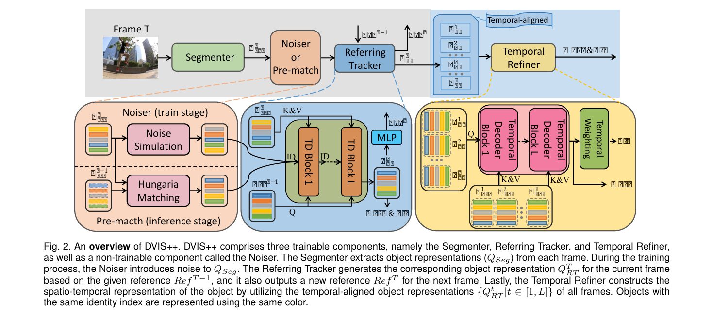
- DVIS++ separates video segmentation into three cascaded stages, a per frame segmenter, a referring tracker, and a temporal refiner, rather than modeling an entire video end to end.
- The referring tracker treats frame to frame association as a denoising problem, and a synthetic noise strategy used only during training is what actually unlocks its tracking accuracy.
- Contrastive learning helps the segmenter and the tracker, but the paper’s own ablation table shows it quietly hurts the temporal refiner on heavily occluded objects even as it improves lightly occluded ones.
- Competing offline methods such as GenVIS and RefineVIS only match strong results in a semi offline, clip by clip mode, and lose several points of accuracy when forced into true offline inference, a distinction easy to miss on a first read of their comparison tables.
- With a frozen CLIP backbone, OV DVIS++ tracks and names object categories such as carrot and kangaroo that never appeared in its training data, at a real cost in accuracy on complex occluded scenes.
The problem with asking one network to do everything
Video segmentation asks a model to find every object in a video, draw a mask around it in each frame, and keep that object’s identity consistent as it moves, gets occluded, and reappears. Video instance segmentation focuses on countable objects like people or animals. Video semantic segmentation focuses on categories like sky or road that do not need individual identities. Video panoptic segmentation asks for both at once. Most research groups build a separate specialized architecture for each of these three tasks, which is expensive to maintain and hard to compare fairly.
A handful of prior attempts at a single unified model, including TarVIS and Tube Link, tried to handle all three tasks with one network, but the paper’s own comparison tables show both trailing well behind specialized methods of the same era. The authors, led by Tao Zhang and Xingye Tian, argue this happens because these systems try to model an object’s full trajectory across an entire video from raw image features in one shot. On a short, simple clip that is manageable. On a long clip full of occlusion and fast motion, the space of possible motion trajectories explodes, and the network has no reliable way to search it.
Offline transformer based methods such as VisTR, SeqFormer, and VITA hit the same wall. They perform well on short benchmark clips but degrade sharply on OVIS, a dataset built specifically to include long videos with heavy occlusion. Online methods that track frame by frame, such as MinVIS and IDOL, avoid that trajectory search problem entirely, but by design they never build a genuine long range spatiotemporal understanding of an object. The paper’s central claim is that neither camp asked the right question. The right question, they argue, is not end to end versus frame by frame. It is how to decompose the task so that each sub problem stays tractable regardless of video length.
Three stages instead of one
DVIS++ breaks video segmentation into three cascaded jobs, each handled by its own trainable module.
The segmenter
The first stage is an ordinary image segmentation network, Mask2Former in the paper’s main configuration, run independently on each frame. It outputs a set of object representations, confidence scores, and pixel masks for that single frame with no awareness of any other frame. This part is treated as a solved problem and is not the paper’s contribution.
The referring tracker
The second stage is the paper’s first real innovation. Rather than treating tracking as a matching problem solved with heuristics like intersection over union or a Hungarian assignment, the referring tracker models it as denoising. Given a reference from the previous frame and the noisy, unordered object representations from the current frame, a stack of transformer blocks learns to reconstruct which current frame object corresponds to which reference. The mechanism doing the real work is what the authors call referring cross attention, where the query and the identity input can be different tensors instead of the standard cross attention setup where they are forced to be the same thing.
The temporal refiner
Once every frame’s objects are aligned to a consistent identity by the tracker, the third stage looks across all the now aligned representations for an entire video and refines both the masks and the category prediction using long range self attention and short range one dimensional convolution. This is only possible because the tracker has already done the hard work of alignment, so the refiner is solving a much simpler problem than trying to model spatiotemporal structure from raw, unaligned frame features.
Mathematical view of referring cross attention
The referring cross attention operation, applied inside each transformer denoising block, is defined below, where ID is the noisy identity input, Q is the reference query, and K and V are the object features from the current frame.
When Q is forced to equal ID, this collapses into a standard cross attention layer, which is exactly the configuration the ablation study tests as a baseline. Swapping in this standard cross attention in place of referring cross attention causes AP on OVIS to fall from 32.8 to 28.3, a drop large enough to make clear that separating the reference signal from the identity signal is doing real work, not just adding parameters.
The denoising training trick that makes the tracker work
Here is a detail that a reader skimming only the abstract would miss entirely, and it turns out to be one of the more interesting engineering decisions in the whole paper. If you feed the tracker object representations that have already been roughly matched by the Hungarian algorithm, which is what happens naturally during inference, the tracker has almost nothing left to learn. Most training clips are simple enough that the Hungarian matching is already close to correct, so the network can achieve very low loss just by copying its input straight through, what the authors call an identity mapping shortcut.
Their fix is to deliberately corrupt the training inputs. During training, a noiser injects synthetic corruption into the object representations before they reach the tracker, using one of three strategies shown in the paper’s Figure 5.
- Random weighted averaging. Each object representation is blended with a randomly chosen different object’s representation using a random mixing weight.
- Random cropping and concatenation. Part of one object’s feature vector is spliced together with part of a different object’s feature vector at a random split point.
- Random shuffling. Object representations are randomly permuted across identities within the frame.
The ablation in the paper’s Table 10 is genuinely surprising. Random shuffling introduces the most extreme corruption of the three, essentially destroying all correspondence between the noisy input and the correct answer, yet it produces the weakest improvement of the three strategies, 33.7 AP versus 35.3 AP for random weighted averaging. The authors’ explanation is that shuffling collapses the sampling space of possible corruptions down to a small number of discrete permutations, while weighted averaging can produce a smoothly varying, effectively infinite range of intermediate corruption levels. The lesson for anyone designing a similar denoising curriculum is that the diversity of the noise distribution matters more than its raw severity.
There is a second counterintuitive result buried in the same table. Extending training from 40,000 to 160,000 iterations with the noise strategy active keeps improving results, gaining another 1.4 AP, and the optimal noise probability shifts upward as training gets longer, from 0.5 to 0.8. A network trained without any synthetic noise plateaus quickly at 33.1 AP no matter how long you train it, because the identity mapping shortcut gives it nothing further to learn.
Where contrastive learning helps, and where it quietly does not
The paper adds a contrastive loss at three points in the pipeline, the segmenter, the referring tracker, and the temporal refiner, each with its own construction of anchor, positive, and negative embeddings. The overall contrastive loss has the standard InfoNCE style form.
Applied to the segmenter, contrastive learning gives a solid 0.8 AP improvement overall, and the gain is heavily concentrated in lightly occluded objects, up 8.0 AP on that subset, with almost no effect on heavily occluded objects, up only 0.4 AP. Applied to the referring tracker as well, the pattern repeats, another 0.7 AP overall with most of the benefit again landing on lightly occluded objects.
Then the paper’s own Table 7 shows something the abstract does not mention at all. Adding contrastive loss to the temporal refiner actually reduces overall AP by 0.6 points compared to the version without it, and the damage is concentrated exactly where the earlier two contrastive losses were strongest, a 2.2 point drop on heavily occluded objects, even though lightly occluded objects improve by 3.3 points. The authors describe this plainly as an unintended consequence, the contrastive objective ends up suppressing the very distinctions between heavily occluded object representations across frames that the temporal refiner needs to correct tracking errors in the first place.
What the comparison tables do not say out loud
Table 1 in the paper marks several competing offline methods, GenVIS, MDQE, NOVIS, and RefineVIS, with a dagger symbol and a footnote explaining that these are semi offline rather than pure offline systems, meaning they process a video in short overlapping clips rather than the entire sequence at once, and that they suffer significant performance degradation when actually run in pure offline mode. The paper states plainly that GenVIS loses roughly 3 AP on YouTube VIS 2021 when forced into true offline inference compared to its reported semi offline numbers.
This matters because a reader comparing headline AP numbers across the table would reasonably assume all offline entries were evaluated the same way. They were not. DVIS++ is one of the only methods in the table that actually improves when run in full offline mode rather than degrading, for example rising from 45.9 to 48.6 VPQ style AP gains on OVIS between its own online and offline configurations, while GenVIS and RefineVIS show flat or negative movement between their semi offline and online numbers. The gap the authors are highlighting is not really DVIS++ against everyone else, it is genuine long range temporal modeling against clip stitching dressed up as offline processing.
Results on the core benchmarks
The following table summarizes online mode, ResNet-50 backbone results across the three VIS benchmarks, taken directly from the paper’s Table 1.
| Method | YouTube VIS 2019 AP | YouTube VIS 2021 AP | OVIS AP |
|---|---|---|---|
| MinVIS | 47.4 | 44.2 | 25.0 |
| IDOL | 49.5 | 43.9 | 28.2 |
| GenVIS | 50.0 | 47.1 | 35.8 |
| TCOVIS | 52.3 | 49.5 | 35.3 |
| DVIS (prior version) | 51.2 | 46.4 | 30.2 |
| DVIS++ | 55.5 | 50.0 | 37.2 |
The gap widens further on OVIS with a frozen VIT-L backbone, where DVIS++ reaches 53.4 AP in offline mode against the previous best result of 45.4 AP from GenVIS, an 8.0 point improvement on precisely the dataset built to stress test occlusion handling. That pattern, a modest edge on the easier YouTube VIS datasets and a much larger edge on the harder OVIS dataset, shows up consistently throughout the paper and is a genuinely useful signal about where this architecture’s advantage actually comes from.
Extending the idea to frozen backbones and open vocabulary
Two further experiments test how far the decoupled design generalizes. The first freezes a DINOv2 pretrained vision transformer entirely and adapts it for dense prediction using a stripped down version of the VIT Adapter, with all injector modules removed to control GPU memory during multi frame training. This lets DVIS++ run on top of a foundation model without any backbone fine tuning, and it still lands competitive results, for example 62.3 AP online on YouTube VIS 2021 with the frozen VIT-L backbone.
The second experiment, OV DVIS++, replaces the segmenter’s backbone with a frozen CLIP encoder in the style of FC-CLIP, letting the whole system classify object categories by comparing visual features against text embeddings rather than a fixed label set. Trained only on COCO images, with zero video specific training data, OV DVIS++ still tracks and correctly names categories it never saw during training, carrot, hay, lantern, kangaroo, in the paper’s qualitative examples.
The zero shot numbers on OVIS reveal an instructive limitation though. When trained only on COCO with ResNet-50, OV DVIS++’s offline mode actually underperforms its own online mode on OVIS, 13.0 AP versus 14.8 AP, the opposite of the pattern seen everywhere else in the paper. The authors attribute this to the pseudo videos generated from COCO images using simple affine transforms being too simplistic, lacking the genuine occlusion and complex motion that the temporal refiner is designed to exploit. Train the temporal refiner on data without real occlusion, and it has little of substance to refine.
Open vocabulary results snapshot
| Method | Backbone | Training data | OVIS zero shot AP |
|---|---|---|---|
| Detic OWTB | ResNet-50 | LVIS | 9.0 |
| MindVLT | ResNet-50 | LVIS | 11.4 |
| FC-CLIP style baseline | ResNet-50 | COCO | 11.8 |
| OV DVIS++ (online) | ResNet-50 | COCO | 14.8 |
What this means going forward
The clearest practical implication for anyone building a video understanding system is that decomposing a hard temporal problem into a chain of tractable sub problems, each with its own supervision signal, can beat throwing more capacity at a single end to end model. That is not a new idea in machine learning generally, but the paper is a well documented case study of it working specifically for video segmentation, complete with the honest admission of where it does not fully hold, particularly under zero shot conditions with unrealistic pseudo video training data.
The denoising formulation of tracking is also worth watching outside video segmentation specifically. Framing an association or matching problem as reconstruction from a corrupted input, then deliberately engineering the corruption distribution during training rather than relying on whatever noise the data happens to contain, is a pattern that could transfer to other sequential association problems such as multi object tracking in robotics or point cloud tracking in autonomous driving.
The failure cases the authors show openly are just as informative as the successes. In one clip, a bird that suddenly takes off and accelerates gets misidentified as a new object because the referring tracker leans on appearance similarity between adjacent frames and has no explicit model of motion or trajectory. In another, the segmenter itself fails to separate two visually near identical zebras standing close together, and no amount of downstream tracking sophistication can fix a mask that was wrong at the source. Both point toward the same conclusion, decoupling made the tracking and refinement stages easier to train well, but it also means the whole system now inherits whatever blind spots exist in the frame level segmenter and in an appearance only association strategy with no motion prior.
Honest limitations
A few constraints are worth keeping in mind before treating these numbers as universally applicable. The training pipeline is staged rather than end to end, the segmenter is trained first and frozen, then the tracker is trained with the segmenter frozen, then the refiner is trained with both earlier stages frozen, specifically to manage GPU memory when handling clips of 21 consecutive frames. This staged approach avoids the memory blowup of true joint training but also means errors introduced early in the segmenter can never be corrected by gradient signal from the later stages during training, only by the temporal refiner’s forward pass at inference time.
The open vocabulary results, while genuinely impressive for a zero shot system, remain well below the fully supervised numbers on the same datasets, 14.8 AP zero shot against 37.2 AP supervised on OVIS with a comparable ResNet-50 backbone, a reminder that open vocabulary generalization still comes at a real accuracy cost on the hardest benchmark. The authors themselves flag that fast motion and visually similar co occurring objects remain unresolved failure modes, and they explicitly propose incorporating trajectory information as a direction for future work rather than claiming the tracking problem is solved.
A reference implementation of the core mechanism
The block below is a simplified, runnable PyTorch implementation of the referring tracker’s denoising mechanism and the temporal refiner’s short term and long term aggregation, built to illustrate the architecture described in Sections 3.2 and 3.3 of the paper. It is not the authors’ original codebase, it is a compact reimplementation meant for learning and experimentation, with a smoke test against random dummy tensors at the end.
import torch
import torch.nn as nn
import torch.nn.functional as F
import random

# ---- Noise simulation strategies (Section 3.4) ----

def random_weighted_average(q: torch.Tensor) -> torch.Tensor:
    # q has shape [N, C]
    n = q.shape[0]
    perm = torch.randperm(n, device=q.device)
    alpha = torch.rand(n, 1, device=q.device)
    return alpha * q + (1 - alpha) * q[perm]

def random_crop_concat(q: torch.Tensor) -> torch.Tensor:
    n, c = q.shape
    perm = torch.randperm(n, device=q.device)
    k = random.randint(1, c - 1)
    out = q.clone()
    out[:, k:] = q[perm][:, k:]
    return out

def random_shuffle(q: torch.Tensor) -> torch.Tensor:
    n = q.shape[0]
    perm = torch.randperm(n, device=q.device)
    return q[perm]

def apply_noise(q: torch.Tensor, strategy: str = "weighted_average", p: float = 0.8) -> torch.Tensor:
    if random.random() > p:
        return q
    if strategy == "weighted_average":
        return random_weighted_average(q)
    elif strategy == "crop_concat":
        return random_crop_concat(q)
    elif strategy == "shuffle":
        return random_shuffle(q)
    raise ValueError("unknown strategy")


# ---- Referring cross attention (Section 3.2, Equation 4) ----

class ReferringCrossAttention(nn.Module):
    def __init__(self, dim: int, heads: int = 8):
        super().__init__()
        self.mha = nn.MultiheadAttention(dim, heads, batch_first=True)

    def forward(self, identity: torch.Tensor, query: torch.Tensor, kv: torch.Tensor) -> torch.Tensor:
        # identity, query, kv all shaped [B, N, C]
        attn_out, _ = self.mha(query, kv, kv)
        return identity + attn_out


class TransformerDenoisingBlock(nn.Module):
    def __init__(self, dim: int, heads: int = 8, ff_dim: int = 1024):
        super().__init__()
        self.rca = ReferringCrossAttention(dim, heads)
        self.norm1 = nn.LayerNorm(dim)
        self.self_attn = nn.MultiheadAttention(dim, heads, batch_first=True)
        self.norm2 = nn.LayerNorm(dim)
        self.ffn = nn.Sequential(nn.Linear(dim, ff_dim), nn.ReLU(), nn.Linear(ff_dim, dim))
        self.norm3 = nn.LayerNorm(dim)

    def forward(self, identity: torch.Tensor, query: torch.Tensor, kv: torch.Tensor) -> torch.Tensor:
        x = self.norm1(self.rca(identity, query, kv))
        attn_out, _ = self.self_attn(x, x, x)
        x = self.norm2(x + attn_out)
        x = self.norm3(x + self.ffn(x))
        return x


class ReferringTracker(nn.Module):
    def __init__(self, dim: int, num_blocks: int = 6, heads: int = 8):
        super().__init__()
        self.blocks = nn.ModuleList([TransformerDenoisingBlock(dim, heads) for _ in range(num_blocks)])
        self.ref_head = nn.Linear(dim, dim)

    def forward(self, ref_prev: torch.Tensor, q_seg: torch.Tensor, noisy_id: torch.Tensor):
        x = noisy_id
        for block in self.blocks:
            x = block(identity=x, query=ref_prev, kv=q_seg)
        new_ref = self.ref_head(x)
        return x, new_ref


# ---- Temporal refiner (Section 3.3) ----

class TemporalDecoderBlock(nn.Module):
    def __init__(self, dim: int, heads: int = 8, kernel_size: int = 3):
        super().__init__()
        self.long_term_attn = nn.MultiheadAttention(dim, heads, batch_first=True)
        self.short_term_conv = nn.Conv1d(dim, dim, kernel_size, padding=kernel_size // 2)
        self.object_self_attn = nn.MultiheadAttention(dim, heads, batch_first=True)
        self.cross_attn = nn.MultiheadAttention(dim, heads, batch_first=True)
        self.ffn = nn.Sequential(nn.Linear(dim, dim * 4), nn.ReLU(), nn.Linear(dim * 4, dim))
        self.norm = nn.LayerNorm(dim)

    def forward(self, q_rt: torch.Tensor, q_seg: torch.Tensor) -> torch.Tensor:
        # q_rt shape [N, T, C]
        n, t, c = q_rt.shape
        long_out, _ = self.long_term_attn(q_rt, q_rt, q_rt)
        x = q_rt + long_out
        short_in = x.transpose(1, 2)
        short_out = self.short_term_conv(short_in).transpose(1, 2)
        x = x + short_out
        x_flat = x.reshape(n * t, 1, c)
        obj_out, _ = self.object_self_attn(x_flat, x_flat, x_flat)
        x = x + obj_out.reshape(n, t, c)
        cross_out, _ = self.cross_attn(x, q_seg, q_seg)
        x = x + cross_out
        return self.norm(x + self.ffn(x))


class TemporalRefiner(nn.Module):
    def __init__(self, dim: int, num_blocks: int = 6, num_classes: int = 40):
        super().__init__()
        self.blocks = nn.ModuleList([TemporalDecoderBlock(dim) for _ in range(num_blocks)])
        self.class_weight = nn.Linear(dim, 1)
        self.cls_head = nn.Linear(dim, num_classes)

    def forward(self, q_rt: torch.Tensor, q_seg: torch.Tensor):
        x = q_rt
        for block in self.blocks:
            x = block(x, q_seg)
        weights = F.softmax(self.class_weight(x), dim=1)
        pooled = (weights * x).sum(dim=1)
        class_logits = self.cls_head(pooled)
        return x, class_logits


# ---- Contrastive loss (Section 3.5, Equation 10) ----

def contrastive_loss(anchor: torch.Tensor, positives: torch.Tensor, negatives: torch.Tensor) -> torch.Tensor:
    pos_sims = anchor @ positives.T
    neg_sims = anchor @ negatives.T
    diff = neg_sims.unsqueeze(-1) - pos_sims.unsqueeze(-2)
    return torch.log1p(torch.exp(diff).sum())


# ---- Smoke test on dummy data ----

def smoke_test():
    dim, n_objects, n_frames = 64, 5, 8

    tracker = ReferringTracker(dim=dim, num_blocks=2)
    refiner = TemporalRefiner(dim=dim, num_blocks=2, num_classes=10)

    ref_prev = torch.randn(1, n_objects, dim)
    aligned_frames = []
    for t in range(n_frames):
        q_seg = torch.randn(1, n_objects, dim)
        noisy_id = apply_noise(q_seg.squeeze(0), strategy="weighted_average", p=0.8).unsqueeze(0)
        q_rt, ref_new = tracker(ref_prev, q_seg, noisy_id)
        aligned_frames.append(q_rt)
        ref_prev = ref_new

    q_rt_all = torch.stack(aligned_frames, dim=2).squeeze(0)
    q_seg_last = torch.randn(n_objects, n_frames, dim)
    refined, class_logits = refiner(q_rt_all, q_seg_last)

    anchor = F.normalize(torch.randn(1, dim), dim=-1)
    positives = F.normalize(torch.randn(3, dim), dim=-1)
    negatives = F.normalize(torch.randn(4, dim), dim=-1)
    loss = contrastive_loss(anchor, positives, negatives)

    assert refined.shape == (n_objects, n_frames, dim)
    assert class_logits.shape == (n_objects, 10)
    assert torch.isfinite(loss)
    print("Smoke test passed.")
    print("Refined shape", refined.shape, "class logits shape", class_logits.shape)
    print("Contrastive loss value", loss.item())

if __name__ == "__main__":
    smoke_test()
Conclusion
DVIS++’s core achievement is proving that a decomposed video segmentation pipeline, with three modules trained in stages and each responsible for a narrow, well defined sub problem, can outperform both specialized single task architectures and prior unified attempts across video instance, semantic, and panoptic segmentation simultaneously. The numbers back this up consistently, from a 3.9 AP jump over the previous best offline method on YouTube VIS 2019 to a much larger 7.5 AP jump on the harder, more occlusion heavy OVIS benchmark, with the gap widening precisely where end to end trajectory modeling struggles most.
The conceptual shift worth taking away is subtler than the leaderboard numbers suggest. The paper is not really arguing that transformers or attention mechanisms are the wrong tool. It is arguing that the way a hard temporal problem gets decomposed before those tools are applied matters as much as the tools themselves, and that a denoising formulation of tracking, trained against deliberately engineered corruption rather than whatever noise happens to occur naturally in a dataset, produces a more robust association mechanism than either heuristic matching or naive learned matching.
That framing plausibly extends beyond video segmentation. Any sequential problem that involves associating entities across time steps under partial occlusion or ambiguity, from multi object tracking in robotics to entity resolution in structured data pipelines, shares the same core difficulty the referring tracker was built to solve. Whether the specific noise simulation strategies used here transfer directly is an open question, but the underlying principle, that identity mapping shortcuts silently cap what a learned association module can achieve unless training deliberately fights them, seems like a durable lesson.
The honest limitations matter just as much as the wins. The staged training process trades end to end optimization for tractable memory usage, the open vocabulary variant still gives up substantial accuracy for zero shot generalization, and the architecture inherits every blind spot of its frame level segmenter along with a tracking mechanism that has no explicit notion of motion. The authors’ own failure case analysis, a bird taking off too fast and a pair of visually near identical zebras, reads as an honest map of where the next version of this work needs to go.
For a research area that has historically been split between specialized architectures that do not generalize and unified architectures that underperform, DVIS++ is a rare case of a unified system actually winning on both counts at once, and its willingness to show exactly where the decomposition strategy still falls short makes it a solid reference point for anyone building the next generation of video understanding systems rather than just another leaderboard entry.
Frequently asked questions
What does DVIS++ actually stand for and what problem does it solve
DVIS stands for Decoupled Video Segmentation. It is a single architecture that handles video instance segmentation, video semantic segmentation, and video panoptic segmentation by splitting the task into a per frame segmenter, a referring tracker, and a temporal refiner instead of using one end to end model.
How is the referring tracker different from a standard object tracker
Most trackers solve an assignment problem using similarity scores and an algorithm like the Hungarian method. The referring tracker instead treats tracking as reconstructing the correct object identity from a deliberately corrupted, noisy input, using a referring cross attention mechanism trained with a synthetic denoising curriculum.
Does contrastive learning always help in this architecture
No. The paper’s own ablation shows contrastive learning helps the segmenter and the referring tracker, especially on lightly occluded objects, but it reduces accuracy when applied to the temporal refiner on heavily occluded objects, a tradeoff the authors document directly rather than gloss over.
Can DVIS++ recognize object categories it was never trained on
Yes, through the open vocabulary variant called OV DVIS++, which uses a frozen CLIP encoder and compares visual features against text embeddings instead of a fixed label set. It correctly tracked categories like carrot and kangaroo in the paper’s qualitative examples despite never seeing them during training, though its accuracy on complex occluded scenes remains well below the fully supervised version.
What are the main known failure cases of DVIS++
The authors show two explicit failure modes, fast moving objects that the appearance based tracker misidentifies as new objects because it has no motion model, and visually near identical objects, such as zebras standing close together, that the frame level segmenter itself fails to separate correctly.
Is DVIS++ trained end to end
No. Because modeling relationships across more than five video frames at once would require prohibitive GPU memory, the segmenter, referring tracker, and temporal refiner are trained in separate stages, with each later stage trained while the earlier stages remain frozen.
Go deeper
Read the full paper for the complete derivations, additional ablations, and qualitative results.
Read the paper on arXiv View the official codeThis analysis is based on the published paper and an independent evaluation of its claims.
Pingback: Revolutionizing Medical Imaging: How a Compact, Programmable Ultrasound Array Unlocks High-Contrast Elastography for Bones and Tumors - aitrendblend.com
Thank you for your sharing. I am worried that I lack creative ideas. It is your article that makes me full of hope. Thank you. But, I have a question, can you help me?
yes please
Thanks for sharing. I read many of your blog posts, cool, your blog is very good. https://www.binance.com/en/register?ref=JHQQKNKN
Your article helped me a lot, is there any more related content? Thanks! https://accounts.binance.com/en-NG/register-person?ref=YY80CKRN
Thanks for sharing. I read many of your blog posts, cool, your blog is very good. https://accounts.binance.bh/it/register/person?ref=P9L9FQKY
Thanks for sharing. I read many of your blog posts, cool, your blog is very good.