
Key points
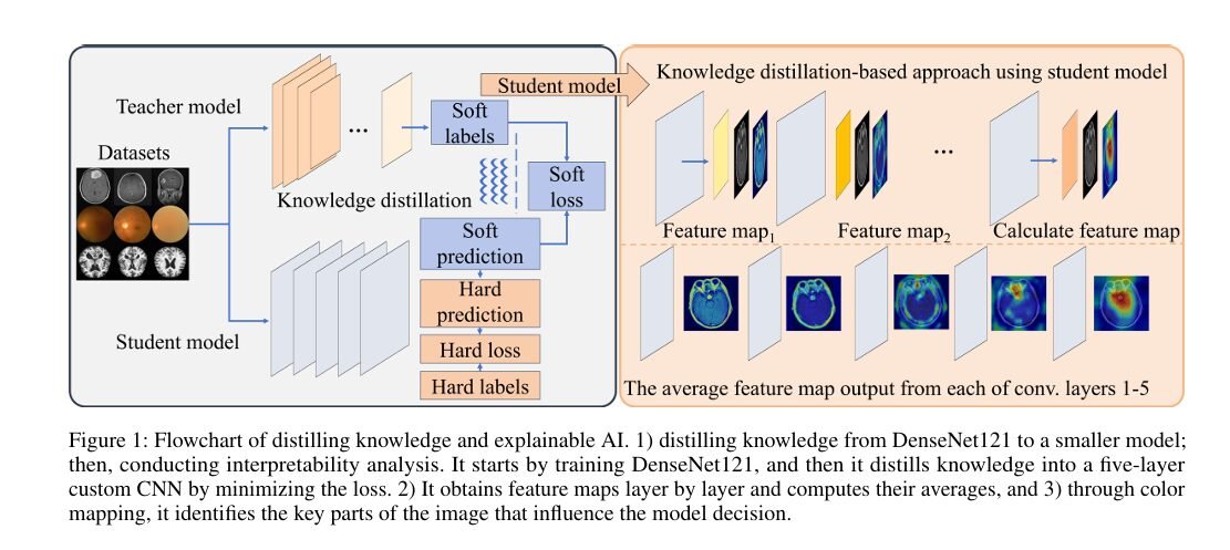
- The team trains a full size DenseNet121 as a teacher, then distills it into a custom student network with only five convolutional layers.
- Instead of running Grad-CAM or SHAP on the heavy teacher, they average the student’s own feature maps layer by layer to show what the network is looking at.
- Across three datasets, brain tumor MRI, eye disease fundus photos and Alzheimer MRI, the student model keeps F1 scores at 0.98, 0.94 and 0.99 respectively.
- The student needs less than half the floating point operations of the teacher and cuts SHAP style analysis time from roughly one minute per image to about fifteen seconds.
- The eye disease dataset is the outlier. The student loses close to five accuracy points against the teacher there, which the paper does not fully explain.
The problem nobody wants to admit about medical AI
Convolutional networks are good at spotting tumors, cataracts and the subtle atrophy patterns that show up in Alzheimer scans. They have been good at this for years. What they are not good at, on their own, is telling a physician which pixels earned that verdict. A model can be right for the wrong reason, and in a hospital that gap between accuracy and trust is not academic. Jin and colleagues, cited in the paper’s introduction, argue that unexplainable results simply do not convince physicians and can contribute to medical accidents when clinicians either over trust a black box or dismiss a genuinely useful signal.
The usual fix is to bolt an explainability method onto a trained model after the fact. Grad-CAM traces gradients back to the last convolutional layer and paints a heatmap. SHAP assigns every input feature a contribution value based on game theory. Both work. Both are also slow when the underlying network is large, and both are explaining a model that was never designed to be understood in the first place. The Guilin team asks a different question. What if the model itself became smaller and simpler before anyone tried to explain it, so that its own internal feature maps could do most of the explaining?
Why knowledge distillation is the tool for the job
Knowledge distillation is not new. Hinton, Vinyals and Dean introduced the idea back in 2015, and it has since become a standard trick for compressing large networks into smaller ones without losing much accuracy. A big teacher network trains normally, then a smaller student network learns to mimic the teacher’s output distribution rather than just the hard ground truth labels. The soft, probability weighted signal from the teacher carries information about which wrong answers are almost right, and that turns out to be a richer training signal than one hot labels alone.
Distillation has already found a home in medical imaging. Termritthikun and colleagues used it to compress chest X ray classifiers for real time multi label diagnosis. Park and colleagues combined distillation with self supervision to diagnose tuberculosis, pneumothorax and COVID 19 even from unlabeled data. Liu and colleagues used a dual branch distillation setup for left ventricular segmentation. What sets the Guilin paper apart is that compression is not the end goal here. It is a means to an interpretability goal. Shrinking the network to five convolutional layers is what makes it feasible to look directly at what each layer is doing, image by image, without drowning in filters.
How the teacher trains the student
The pipeline starts with DenseNet121, pretrained on ImageNet, fine tuned separately on each of the three medical datasets to serve as the teacher. The student is a much shallower custom convolutional network, five layers deep, trained from scratch under two loss signals at once.
The first is a familiar hard loss, ordinary cross entropy between the student’s predictions and the true one hot labels.
The second is a soft loss that compares the student’s temperature scaled predictions against the teacher’s temperature scaled predictions, which is effectively a cross entropy between two softened probability distributions rather than between predictions and hard labels.
A temperature parameter \(T\) controls how soft that distribution gets. Push \(T\) higher and the differences between the largest and smallest class probabilities shrink, which highlights relative confidence rather than a single overconfident spike. The two losses combine into one training objective through a weighting term \(\alpha\).
The teacher uses average pooling during training to preserve background context, while the student switches to max pooling so it grabs the sharpest, most prominent activation in each region. That single architectural choice matters more than it sounds. Average pooling smooths detail away. Max pooling keeps the loudest signal, which is exactly what you want when the whole point of the exercise is to trace which pixels the network cared about.
Turning feature maps into pictures a clinician can read
Once the student model exists, the authors do not run Grad-CAM or SHAP on it as the primary explanation method. Instead they pull the raw activation maps out of each convolutional layer and average them across all filters in that layer.
Here \(F_k(i,j)\) is the activation value at position \((i,j)\) produced by the \(k\) th filter, and \(N\) is the total filter count in that layer. A convolutional layer with, say, sixty four filters would normally produce sixty four separate 2D maps for a single input image, which is far too many for a human to scan through one at a time. Averaging collapses that stack into one map per layer, five maps total for a five layer student, each one colored and overlaid on the original scan.
The result reads like a flipbook of how the network’s attention narrows as it goes deeper. Early layers pick up on gross structure, the outline of a brain or the round shape of a fundus photo. Middle layers start isolating textures and local shapes. By the fourth and fifth layers, the highlighted region increasingly lines up with the actual clinical area of interest, the tumor mass, the optic disc, the ventricles.
Key takeaway
The interpretability method here is not an add on explainer bolted to a finished model. It is a byproduct of the architecture itself. Because the student only has five layers, showing every layer’s average feature map is actually feasible, which is the entire reason the compression step comes first.
What the numbers actually show
The team tested this pipeline on three public datasets. Brain tumor MRI combines the figshare, SARTAJ and Br35H collections into 7023 images across four classes, glioma, meningioma, no tumor and pituitary. Eye disease uses 4217 color fundus photographs split into cataract, diabetic retinopathy, glaucoma and normal. Alzheimer draws on an augmented MRI set with 8960 mild, 6464 moderate, 9600 non demented and 8960 very mild demented images. Training ran on a single RTX 4090 with TensorFlow, the Adam optimizer, a learning rate of 1 times 10 to the negative fourth power, and a batch size of sixteen.
| Dataset | Teacher accuracy | Best student accuracy | Best student setting | Student avg F1 |
|---|---|---|---|---|
| Brain tumor | 0.9877 | 0.9748 | alpha 0.7, T 10 | 0.98 |
| Eye disease | 0.9837 | 0.9351 | alpha 0.4, T 15 | 0.94 |
| Alzheimer | 0.9938 | 0.9946 | alpha 0.4, T 5 | 0.99 |
Two of those rows are the headline result. On brain tumor MRI the five layer student loses only about one accuracy point against a full DenseNet121. On the Alzheimer dataset the student actually edges past its teacher, 0.9946 against 0.9938, which the authors attribute to a favorable temperature setting that let the student absorb useful signal faster than the harder one hot labels would have allowed on their own.
The eye disease row tells a different story and the article would be dishonest to gloss over it. The best student there trails the teacher by close to five accuracy points, 0.9351 against 0.9837. Four classes that hinge on subtle vascular and structural differences around the optic disc apparently need more representational depth than five convolutional layers can offer. The paper states this plainly as a limit of shallow networks, without pretending the compression was free everywhere.
Comparing the new method against Grad-CAM and SHAP
To check whether the layer by layer feature maps actually mean anything, the authors computed a fidelity score for each explanation method. The formula compares a model’s confidence on an adversarially perturbed image against its confidence on the original image for the true class.
| Dataset average | Grad-CAM | SHAP | This method |
|---|---|---|---|
| Brain tumor | 0.9298 | 0.9404 | 0.9277 |
| Eye disease | 0.9059 | 0.8700 | 0.8630 |
| Alzheimer | 0.9112 | 0.9359 | 0.9132 |
SHAP wins on fidelity in two of the three datasets, and by a wide margin on Alzheimer scans, where symptoms are spread across many brain regions and SHAP’s per feature accounting captures that diffuseness well. The new layer averaging method lands close behind Grad-CAM in every case rather than beating it outright. That is a fair result rather than a flattering one, and the paper is upfront that its method broadly mirrors what Grad-CAM and SHAP already find instead of surpassing them on this particular metric.
Where the new method pulls ahead is speed, and the gap is not small.
| Model | FLOPs (millions) | Grad-CAM time | SHAP time |
|---|---|---|---|
| Teacher (DenseNet121) | 566.89 | about 0.93 to 0.95 seconds | about 67.6 to 68.5 seconds |
| Student (five layer CNN) | 232.70 | about 0.19 to 0.20 seconds | about 15.4 to 15.6 seconds |
The student needs less than half the floating point operations of the teacher, and that difference compounds badly for SHAP, which already scales poorly with model complexity because it has to test many feature combinations. A method that takes roughly one minute per image on the teacher drops to about fifteen seconds on the student. For a single scan that is a nice convenience. For a hospital running batch analysis on hundreds of images overnight, that is the difference between a report that is ready by morning and one that is not.
Key takeaway
Fidelity and speed are two separate wins and the paper does not conflate them. The new method is not the most faithful explanation available, SHAP usually is. It is the fastest one that still holds up reasonably well, which matters most exactly when a clinic needs to explain many images quickly rather than one image perfectly.
Clinical translation gap
None of this has been tested in an actual clinical workflow. The datasets here are curated, labeled research collections, not the messy, inconsistent scans that come off real hospital scanners with real patient variability, motion artifacts and equipment differences. A model trained on the SARTAJ or Br35H brain tumor collections has not seen the imaging protocols of every hospital that might eventually want to use it, and generalization from a research benchmark to a specific clinical site is never guaranteed. The paper also does not report how the average feature maps were validated against an actual radiologist’s read of the same scans, only against Grad-CAM and SHAP run on the teacher model, which are themselves approximations rather than ground truth about what a clinician would circle by hand. A tool built for speed and shallow architecture is genuinely useful for research triage and rapid screening pipelines, but the leap from a validated benchmark to a bedside decision support tool involves regulatory review, prospective clinical trials and the kind of dataset diversity this study, built on three fixed public collections, does not attempt to cover.
Why this matters beyond radiology
Step back from the specific datasets and the pattern here generalizes. Any field using large convolutional networks for classification, from satellite imagery to industrial defect detection, faces the same tension between accuracy and explainability. This paper’s contribution is really a workflow. Train a strong teacher, distill it down until its layers are few enough to inspect directly, then let the model’s own architecture do the explaining instead of layering a separate explainer on top after the fact.
That said, the eye disease result is a useful caution against assuming this workflow generalizes for free. Some tasks need the representational capacity that comes with depth, and forcing a five layer student onto a problem that needs sixteen or fifty layers will cost real accuracy. The honest reading of this paper is not that shallow students always work. It is that shallow students are worth trying first, and worth abandoning quickly when the accuracy gap gets too wide, which is exactly what happened with the eye disease dataset here.
Limitations worth sitting with
Three limitations stand out beyond the ones the authors state directly. First, sample sizes vary widely by class within each dataset. Diabetic retinopathy has 1098 images while glaucoma has 1007, a fairly even split, but within Alzheimer, moderate demented sits at 6464 images against non demented at 9600, an imbalance that can quietly bias a classifier toward the majority class even when overall accuracy looks strong. Second, all three datasets come from public repositories that have been used repeatedly across the explainability literature, which raises the ordinary risk that models and hyperparameters have been implicitly tuned toward quirks specific to these exact collections rather than toward medical imaging broadly. Third, the fidelity score itself depends on how adversarial perturbations are generated, and the paper does not detail the perturbation budget or method in enough depth for an independent group to reproduce the exact numbers without consulting the code repository directly.
None of that erases the result. It does mean a hospital evaluating this approach should treat the reported numbers as a starting point for its own validation rather than as evidence that is ready to deploy as is.
Read the full paper for the complete architecture details, training curves and additional visualizations.
Conclusion
The core achievement here is modest sounding but useful. A five layer student network, trained through standard knowledge distillation from a DenseNet121 teacher, keeps accuracy within roughly one point of the teacher on brain tumor MRI and actually edges past it on Alzheimer MRI, while needing less than half the compute and cutting SHAP style analysis time by a factor of roughly four. That is a real, measurable gain for anyone building a screening pipeline that needs to move fast without abandoning interpretability.
The conceptual shift matters more than any single accuracy number. Instead of treating explainability as something applied to a finished, opaque model after training ends, this paper treats it as a design constraint that shapes the model from the start. Compress first, then let the compressed model’s own structure carry the explanation. That inverts the usual order of operations in most explainable AI work, where a heavy model gets trained for accuracy and an explainer gets bolted on afterward almost as an afterthought.
Whether this transfers cleanly to other domains is an open question the paper does not directly test, but the underlying idea, that a smaller model is not just cheaper but genuinely easier to interrogate, has obvious appeal for any classification task under real time or resource constraints. Anywhere a practitioner currently tolerates a slow, bolted on explainer because the base model is too large to inspect directly, this workflow offers an alternative worth benchmarking.
The honest limitations remain real. The eye disease result shows shallow students are not a universal fix, class imbalance within the Alzheimer set deserves closer scrutiny, and nothing here has been through clinical validation on real hospital data. A method that works well on three specific public datasets under one set of hyperparameters has not yet proven it works everywhere, and the authors do not claim otherwise.
What the paper does establish, carefully and with real numbers rather than vague optimism, is that the tradeoff between a model being right and a model being understandable does not have to be as steep as the field has generally assumed. Sometimes making the model smaller is the fastest path to making it honest about how it reached its answer, and that is a genuinely useful lesson for anyone building AI systems that people need to trust rather than simply obey.
Frequently asked questions
What is knowledge distillation in simple terms
It is a training technique where a small student network learns to copy the output patterns of a larger, already trained teacher network, rather than learning only from the original labeled data. The student ends up smaller and faster while keeping most of the teacher’s accuracy.
Why does a smaller model help with explainability
A smaller network has fewer layers and filters to inspect, so techniques like averaging feature maps across all filters in a layer become practical to compute and simple enough for a human to read, which is much harder to do cleanly on a network with dozens of layers.
How accurate is the student model compared to the original DenseNet121
It varies by dataset. On brain tumor MRI the student reached 0.9748 accuracy against the teacher’s 0.9877. On Alzheimer MRI the student actually reached 0.9946, slightly above the teacher’s 0.9938. On eye disease images the student dropped to 0.9351 against the teacher’s 0.9837, a noticeably larger gap.
Is this method better than Grad-CAM or SHAP
Not on the fidelity metric the paper reports, where SHAP scored highest in two of three datasets and Grad-CAM edged ahead in one. The new method’s advantage is speed. It cuts SHAP style analysis time from roughly one minute per image to about fifteen seconds while producing broadly similar visual explanations.
Has this been tested in a real hospital
No. The study uses three public research datasets, not live clinical data, and the authors do not report deployment or validation in an actual clinical workflow. This is early stage research, not a cleared medical device.
Where can I find the code for this project
The authors published their implementation on GitHub under the name KD-FMV, linked in the CTA section above and cited directly in the paper.
Related Posts
Reference implementation
The block below is an independent PyTorch reimplementation of the teacher student pipeline and the feature map averaging step described in the paper. It is written for clarity and to run a quick smoke test on random dummy tensors, not copied from the authors’ TensorFlow codebase linked above.
# kd_fmv.py
# Independent PyTorch reimplementation of the teacher student distillation
# pipeline and layer wise average feature map extraction described in
# "A Knowledge Distillation Based Approach to Enhance Transparency of
# Classifier Models" (arXiv 2502.15959). Written for aitrendblend.com.

import torch
import torch.nn as nn
import torch.nn.functional as F
from torch.utils.data import DataLoader, TensorDataset
from torchvision.models import densenet121
from sklearn.metrics import f1_score


class TeacherModel(nn.Module):
    """DenseNet121 backbone, pretrained on ImageNet, head resized to the
    number of target classes for a given dataset."""

    def __init__(self, num_classes=4, pretrained=True):
        super().__init__()
        base = densenet121(weights="IMAGENET1K_V1" if pretrained else None)
        in_features = base.classifier.in_features
        base.classifier = nn.Linear(in_features, num_classes)
        self.net = base
        # the paper uses average pooling in the teacher to preserve
        # background context, torchvision densenet already does this
        # in its final classifier head via adaptive average pooling

    def forward(self, x):
        return self.net(x)


class StudentCNN(nn.Module):
    """Five convolutional layer student network with max pooling,
    matching the shallow architecture used for the feature map
    visualization stage in the paper."""

    def __init__(self, num_classes=4, in_channels=3):
        super().__init__()
        channels = [32, 64, 128, 256, 256]
        layers = []
        prev = in_channels
        for ch in channels:
            layers.append(nn.Conv2d(prev, ch, kernel_size=3, padding=1))
            layers.append(nn.BatchNorm2d(ch))
            layers.append(nn.ReLU(inplace=True))
            layers.append(nn.MaxPool2d(2))  # max pooling, per the paper
            prev = ch
        self.blocks = nn.ModuleList(layers)
        self.pool = nn.AdaptiveAvgPool2d(1)
        self.classifier = nn.Linear(channels[-1], num_classes)

    def forward(self, x, return_feature_maps=False):
        feature_maps = []
        h = x
        for layer in self.blocks:
            h = layer(h)
            if isinstance(layer, nn.MaxPool2d):
                feature_maps.append(h)  # one snapshot per conv block
        pooled = self.pool(h).flatten(1)
        logits = self.classifier(pooled)
        if return_feature_maps:
            return logits, feature_maps
        return logits


def average_feature_map(feature_map):
    """Implements A(i, j) = (1 / N) * sum_k F_k(i, j) from the paper,
    collapsing all filters in a layer into one 2D map per image."""
    # feature_map shape is (batch, channels, height, width)
    return feature_map.mean(dim=1)  # average across the filter dimension


def distillation_loss(student_logits, teacher_logits, targets, alpha=0.4, temperature=10.0):
    """Combines hard cross entropy loss with a temperature scaled soft
    loss between student and teacher outputs, matching Eq. 1 to Eq. 3
    in the paper."""
    hard_loss = F.cross_entropy(student_logits, targets)

    student_soft = F.log_softmax(student_logits / temperature, dim=-1)
    teacher_soft = F.softmax(teacher_logits / temperature, dim=-1)
    soft_loss = F.kl_div(student_soft, teacher_soft, reduction="batchmean") * (temperature ** 2)

    return alpha * hard_loss + (1 - alpha) * soft_loss


def train_student(teacher, student, dataloader, epochs=5, alpha=0.4, temperature=10.0, lr=1e-4, device="cpu"):
    teacher.eval()
    student.to(device)
    teacher.to(device)
    optimizer = torch.optim.Adam(student.parameters(), lr=lr)

    for epoch in range(epochs):
        student.train()
        running_loss = 0.0
        for images, targets in dataloader:
            images, targets = images.to(device), targets.to(device)

            with torch.no_grad():
                teacher_logits = teacher(images)

            student_logits = student(images)
            loss = distillation_loss(student_logits, teacher_logits, targets, alpha, temperature)

            optimizer.zero_grad()
            loss.backward()
            optimizer.step()
            running_loss += loss.item()

        print(f"epoch {epoch + 1} average loss {running_loss / len(dataloader):.4f}")

    return student


def evaluate(model, dataloader, device="cpu"):
    model.eval()
    all_preds, all_targets = [], []
    correct, total = 0, 0
    with torch.no_grad():
        for images, targets in dataloader:
            images, targets = images.to(device), targets.to(device)
            logits = model(images)
            preds = logits.argmax(dim=1)
            correct += (preds == targets).sum().item()
            total += targets.size(0)
            all_preds.extend(preds.cpu().tolist())
            all_targets.extend(targets.cpu().tolist())

    accuracy = correct / total
    f1 = f1_score(all_targets, all_preds, average="macro")
    return {"accuracy": accuracy, "f1": f1}


def smoke_test():
    """Runs the full pipeline on random dummy tensors so the wiring
    between teacher, student, loss and evaluation can be checked
    without downloading any real dataset."""
    torch.manual_seed(0)
    num_classes = 4
    batch_size = 8
    dummy_images = torch.randn(32, 3, 128, 128)
    dummy_labels = torch.randint(0, num_classes, (32,))
    dataset = TensorDataset(dummy_images, dummy_labels)
    loader = DataLoader(dataset, batch_size=batch_size, shuffle=True)

    teacher = TeacherModel(num_classes=num_classes, pretrained=False)
    student = StudentCNN(num_classes=num_classes)

    student = train_student(teacher, student, loader, epochs=2, alpha=0.4, temperature=10.0)
    metrics = evaluate(student, loader)
    print("dummy data metrics", metrics)

    sample_images, _ = next(iter(loader))
    _, feature_maps = student(sample_images, return_feature_maps=True)
    for idx, fmap in enumerate(feature_maps, start=1):
        avg_map = average_feature_map(fmap)
        print(f"layer {idx} average feature map shape", avg_map.shape)


if __name__ == "__main__":
    smoke_test()
The smoke test above builds both models with random weights, runs two training epochs on random tensors purely to confirm the loss and optimizer wiring works, then pulls the average feature map out of each of the five student layers to confirm the shapes match what a real image batch would produce. Swap the dummy tensors for a real dataset loader and the pipeline mirrors the one described in the paper closely enough to reproduce the same overall training loop, even though the exact TensorFlow implementation the authors used is linked above.
This analysis is based on the published paper and an independent evaluation of its claims.
Pingback: MedDINOv3: Revolutionizing Medical Image Segmentation with Adaptable Vision Foundation Models - aitrendblend.com
Thank you for your sharing. I am worried that I lack creative ideas. It is your article that makes me full of hope. Thank you. But, I have a question, can you help me?
Thank you for your sharing. I am worried that I lack creative ideas. It is your article that makes me full of hope. Thank you. But, I have a question, can you help me?