
Key points
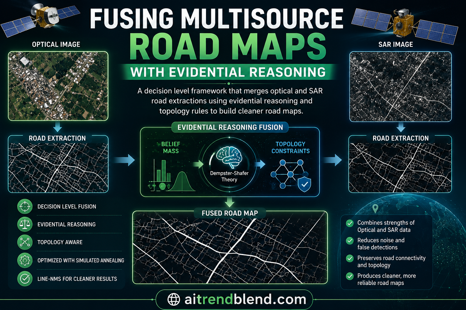
- Researchers from the University of Electronic Science and Technology of China built a two stage decision level fusion framework that merges road extractions from multiple remote sensing sources without needing a single jointly trained model.
- Stage one, called Line-NMS, is a geometry driven algorithm adapted from nonmaximum suppression that removes duplicate road segments where different sources overlap.
- Stage two fuses the surviving evidence using the evidential reasoning rule, weighting each source by measured reliability, then folds in road topology as part of one energy function solved with simulated annealing.
- On multitemporal optical imagery the fused result reached an overall quality score of 60.52 percent, beating six other decision level fusion methods on that composite metric while keeping redundancy far lower than the simplest baseline.
- On fused optical and SAR imagery, correctness jumped from 73.43 percent for optical alone to 88.16 percent after fusion, with quality improving from 56.49 percent to 66.34 percent.
- An ablation study confirms that geometry based deduplication, evidential fusion, and topology constraints each contribute separately, and the full combination outperforms any subset of the three.
Why one sensor is never quite enough
Extracting road networks automatically from satellite and airborne imagery has been a live research problem for decades, and the authors note that a search of the Web of Science database turns up roughly ten thousand papers on the topic. The overwhelming majority, by their count around ninety percent, work from a single imaging source. That is a real limitation. Optical imagery is at the mercy of weather, cloud cover, and the shadows cast by buildings and trees. Synthetic aperture radar avoids those problems since it can see through clouds and works day or night, but it introduces its own headaches, chiefly speckle noise and geometric distortion that make road boundaries fuzzy in a different way.
The obvious fix is to combine sources so each one’s weaknesses get covered by the other’s strengths. The obvious fix is also harder than it sounds. Coregistered, jointly labeled multisource datasets are expensive to build and rare to find, and training one model to consume several sensor types at once tends to produce a brittle system that has to be retrained whenever the combination of inputs changes. That is why this paper focuses on decision level fusion instead, combining the outputs of separately trained, already existing models rather than building one model that ingests everything at once.
What decision level fusion buys you
Data fusion in remote sensing is usually split into three levels. Raw data fusion combines pixel values before any interpretation happens. Feature level fusion combines the intermediate representations a model builds internally. Decision level fusion waits until each source has already produced its own answer, in this case a candidate road map, and combines those finished answers. The tradeoff is that decision level methods give up some of the accuracy a tightly coupled feature level model can achieve, but they gain enormous flexibility. You can swap in a new sensor, a new segmentation model, or a differently trained version of an existing model without retraining anything else in the pipeline.
Existing decision level approaches for road extraction have generally been simple to the point of being blunt. Logical OR fusion just stacks every candidate road pixel from every source together, which recovers a lot of true road but drags along a large amount of duplicated, overlapping detections. Majority voting and Borda count schemes are easy to implement but ignore how reliable any particular source actually is. Bayesian and evidence theory approaches do better by modeling uncertainty explicitly, but classical Dempster Shafer theory, a common choice in this space, treats every source as equally trustworthy by default and behaves oddly when two sources strongly disagree.
A two stage pipeline built around structure, not just probability
The framework starts with data preparation that sits outside the paper’s main contribution. Multisource images get registered to a common coordinate frame using an affine transformation with manually selected control points, then each source is run through its own road segmentation model to produce a binary road map and a pixel level confidence map. The team used two different segmentation architectures across their experiments, DLinkNet34 and MSMDFF-Net, deliberately choosing distinct model families to test whether the fusion framework generalizes across segmentation paradigms rather than being tuned to one specific network. The segmented maps are then thinned down to skeleton line segments using a centerline extraction method the authors developed in earlier work, since working with vectorized line segments rather than raw pixel masks keeps the downstream fusion computationally manageable and makes it far easier to reason about road topology.
From there the real contribution begins, a two stage decision fusion process. The first stage cleans up geometric redundancy. The second stage combines the surviving evidence using the evidential reasoning rule while simultaneously enforcing that the final road network actually looks like a road network, connected, without stray dangling fragments, with junctions that resemble real intersections.
Stage one, redundancy removal with Line-NMS
Because every source is looking at the same geographic area, overlapping road segments from different sources are common and expected. The authors adapted a familiar idea from object detection, nonmaximum suppression, to work on linear features instead of bounding boxes, and named the result Line-NMS.
The algorithm repeatedly selects the longest remaining line segment across all sources, keeps it, then checks every other segment against it using two geometric measures. The included angle between two segments tells the algorithm whether they are pointing in roughly the same direction. The overlap ratio tells it how much of a shorter segment’s length actually sits within a dilated buffer around the longer one. If a candidate segment is close enough in angle and overlaps enough with the segment already kept, it gets merged away as redundant rather than duplicated in the output. A threshold on the angle search range is fixed at one eighth of pi throughout the paper, while the overlap threshold shrinks adaptively as segments get shorter, so that small fragments are held to a stricter redundancy standard than long, confident road stretches.
Here card counts pixels, e_2^{ex} is a dilated version of the second segment sized to its detected road width, and the ratio measures what fraction of the first segment actually falls inside that dilated buffer. After Line-NMS runs, a separate junction regularization step based on spline fitting cleans up the intersections and endpoints that thinning and merging tend to scatter slightly out of alignment, snapping nearby endpoints together into single, coherent junctions.
Turning the road network into a graph
To bring topology into the fusion process, the surviving line segments get converted into a proper graph. The pipeline detects every intersection and segments the network there, then applies the Douglas Peucker curve simplification algorithm within each connected piece to find internal turning points and split further at those locations. What remains are edges with low curvature, connected at vertices that represent real intersections, endpoints, and turning points.
Once the graph exists, two structural features get computed for every edge. The degree of each vertex, simply how many edges meet there, distinguishes a dead end from a normal two way connection from a busy four way or more intersection. Each edge also gets a normalized length and an angle attribute describing how sharply it bends relative to its neighbors. These numbers are what let the energy function penalize configurations that look geometrically implausible for a real road network later on.
Fusing evidence with the evidential reasoning rule
The second stage is where the paper’s central idea lives. Rather than treating each source’s confidence score as a ready made probability, the authors treat it as raw, potentially biased evidence that needs calibration before it can be trusted.
Learning belief probability functions from data
Each road candidate segment gets classified into one of three states under the frame of discernment used by evidential reasoning theory, road, non road, or uncertain. Rather than assuming any particular functional shape, the team builds a histogram of confidence scores against ground truth labels for each source, then fits a sigmoid shaped curve to that histogram using nonlinear least squares solved with the Levenberg Marquardt algorithm. They argue this fits the real distribution of confidence scores better than the trapezoidal belief functions common in earlier evidence theory work, and the fitted curves in the paper’s figures do track the underlying histograms closely.
The practical payoff of this calibration step is that once the four parameters per source are fit on a training set, they transfer to new images acquired by the same sensor and model without needing to be refit each time, which matters a great deal for a framework meant to keep working as new imagery arrives.
Combining sources that do not trust each other equally
With calibrated belief probabilities in hand, the evidential reasoning rule combines evidence from each source while explicitly accounting for two separate properties, reliability and weight. Reliability is treated as an intrinsic property of a source, essentially how good that source’s model has historically been at getting the right answer, and in this paper it is estimated directly from each segmentation model’s F1 score on a held out test set. Weight is a separate, more subjective knob representing how much importance the operator wants to assign a given source, useful for deliberately favoring a higher resolution sensor over a lower resolution one even if their raw accuracy is similar.
This separation is the specific advance over classical Dempster Shafer combination, which folds everything into one normalization step and can produce counterintuitive results when two sources disagree sharply. By redistributing conflicting evidence according to each source’s credibility rather than discarding it uniformly, the evidential reasoning rule tends to behave more sensibly under exactly the kind of disagreement multisource fusion is bound to produce.
What reliability and weight actually control
Reliability answers the question how good is this source generally, estimated empirically from performance metrics. Weight answers the question how much should this source matter to me right now, set by the operator based on domain knowledge such as sensor resolution or acquisition conditions. Keeping these two ideas separate rather than collapsing them into one confidence number is what lets the framework favor a more informative source without also having to pretend that source is infallible.
Making the fusion topology aware
A pure evidence fusion step still has no concept of what a road network should look like structurally. It can confidently label a two pixel fragment as road even though that fragment connects to nothing. To close that gap, the authors define a single energy function over the whole graph that combines the evidential fusion result with explicit topological penalties, then solve for the labeling that minimizes it.
The observation term rewards labelings that agree with the fused belief probabilities from the evidential reasoning stage. The priori term penalizes structurally unreasonable configurations, isolated segments dangling off nothing, short burrs branching from the main network, and intersections with implausible numbers of connected roads. Four positive parameters control how aggressively each of these penalties bites, and the authors set them once based on general road network characteristics rather than tuning them per dataset, reporting values that held up across both of their test regions. The weighting term gamma balances how much the final answer leans on raw evidence versus structural plausibility, and a sensitivity sweep across both case studies points to an optimal value near 0.3.
Solving for the labeling that minimizes this energy function is a combinatorial problem, since every edge in the graph could in principle be either road or non road, so the authors turn to simulated annealing, starting every edge labeled as road and letting the algorithm cool down over up to five thousand iterations while occasionally accepting worse solutions to escape local minima. This is a deliberate and reasonable choice for a landscape with this many local optima, though it is also the main reason the fusion stage takes noticeably longer to run than the simpler baselines it is compared against.
Testing it on real satellite and radar imagery
The team ran two case studies covering the two most common multisource scenarios in the field, images of the same place taken at different times, and images of the same place taken by different sensor types.
Case study one, two optical scenes months apart
The first test used two Jilin-1 optical images of Wulan, Qinghai, captured in November 2021 and April 2022 at 0.75 meter resolution. Seasonal vegetation changes and shifting shadow angles between the two dates produced noticeably different segmentation results even though the same MSMDFF-Net model, trained on the DeepGlobe dataset, processed both images.
| Source | Completeness | Correctness | Quality | Redundancy |
|---|---|---|---|---|
| November 2021 image alone | 68.68 percent | 69.35 percent | 52.69 percent | 0.0094 |
| April 2022 image alone | 74.91 percent | 70.09 percent | 56.77 percent | 0.0086 |
| Both images fused | 77.58 percent | 73.35 percent | 60.52 percent | 0.0056 |
Fusing the two dates beat either single date on every metric at once, which is a meaningful result since it is common for a fusion method to trade one metric for another rather than improving everything simultaneously. Against six other decision level fusion baselines, the framework achieved the highest overall quality score among methods with low redundancy. Logical OR fusion technically posted a higher completeness and quality figure, but only by accepting a redundancy score more than sixty times higher, essentially by keeping every duplicate detection rather than resolving them, which the authors rightly treat as a hollow win rather than a genuine advantage.
Case study two, optical paired with radar
The second test fused Gaofen-3 SAR imagery with HH polarization against a corresponding Google Earth optical image over Jiujiang, Jiangxi, using the FUSAR-Map dataset at one meter resolution, with D-LinkNet34 trained separately on each modality.
| Source | Completeness | Correctness | Quality | Redundancy |
|---|---|---|---|---|
| Optical image alone | 71.00 percent | 73.43 percent | 56.49 percent | 0.0031 |
| SAR image alone | 44.02 percent | 54.39 percent | 32.15 percent | 0.0106 |
| Optical and SAR fused | 72.83 percent | 88.16 percent | 66.34 percent | 0.0036 |
SAR performed considerably worse than optical on its own here, unsurprising given how much noisier radar backscatter tends to be over dense urban texture. What stands out is how much correctness improved after fusion, jumping more than fourteen percentage points past optical alone, evidence that the SAR channel is contributing real complementary information even though its standalone performance is comparatively weak. The reliability values estimated for each source in this experiment, 0.72 for optical and 0.52 for SAR based on each model’s F1 score, and the operator assigned weights, 1.0 for optical and 0.7 for SAR reflecting its lower resolution, both fed directly into how much influence each source carried during evidential fusion. Against the same six baseline methods, the framework again produced the best overall quality score while keeping redundancy among the lowest of any method tested.
What the ablation study shows about each piece
Because the framework has three logically separable components, geometric redundancy removal, evidential fusion, and topology constraints, the authors ran an ablation study isolating each one’s contribution across both case studies.
| Components active | Case study I quality | Case study II quality |
|---|---|---|
| Geometric fusion alone | 54.60 percent | 61.13 percent |
| Geometric fusion plus evidential reasoning | 56.39 percent | 61.79 percent |
| Geometric fusion plus topology constraints | 59.14 percent | 64.42 percent |
| Full framework, all three components | 60.52 percent | 66.34 percent |
Every added component improved the overall quality score in both case studies, and the full combination beat any subset. Evidential reasoning alone tended to raise correctness noticeably while depressing completeness, since filtering by source credibility naturally throws out some borderline true detections along with genuine noise. Topology constraints alone moved the needle less dramatically per component but preserved a healthier balance between completeness and correctness. Only together do the three pieces produce the best composite result, which is a reasonably convincing argument that this is a case where the whole genuinely exceeds the sum of its parts rather than one dominant component carrying the other two.
The honest tradeoff, accuracy against running time
The proposed method’s biggest weakness relative to its competitors is speed. On the multitemporal test it took 387.57 seconds compared to well under two minutes for every other method except the simplest logical OR baseline, which finishes in a fraction of a second by doing essentially no work. That gap comes almost entirely from the simulated annealing optimization at the core of stage two, and the authors are upfront that this limits how directly the current implementation could serve large scale or genuinely real time applications without further engineering, pointing to parallelized patch processing or faster combinatorial solvers such as graph cuts as likely paths forward.
What this framework changes about how road fusion gets approached
Most existing decision level fusion work for road extraction either ignores topology entirely or bolts it on afterward as a cleanup pass applied to an already finalized road map. This paper’s central bet is that topology belongs inside the optimization from the start, expressed as one term in the same energy function that the evidential fusion result feeds into, rather than as a second, disconnected postprocessing stage. The ablation results back that choice up reasonably well, since topology constraints contributed real, measurable gains on their own and additional gains on top of evidential fusion rather than simply cleaning up its output after the fact.
The broader pattern here, calibrating each source’s raw confidence output into a properly fit belief function before fusing anything, is worth noting outside road extraction specifically. Any decision level fusion task that combines outputs from differently trained, differently biased models faces the same underlying problem this paper solves for roads, namely that a model’s raw softmax or confidence score is rarely a trustworthy probability on its own. Fitting a calibration curve per source before combining evidence is a comparatively cheap step that this paper shows can meaningfully change downstream fusion quality.
Honest limitations
Running time is the most concrete limitation, and the authors do not shy away from it. A method that takes over six minutes per fusion pass on the reported hardware is not yet a drop in replacement for a fast baseline in a genuinely time sensitive pipeline, even if the quality gain justifies the cost for offline database updating. The topology penalty parameters, while shown to generalize reasonably across two different urban test regions, were set once based on general characteristics of road networks rather than learned from data, and the authors themselves note they may need further tuning for road networks with substantially different spatial patterns or densities than the ones tested here. The evaluation also covers exactly two case studies, one multitemporal and one multimodal, both over urban Chinese cities, which is a reasonable proof of concept but a limited basis for claiming the framework generalizes to, say, rural road networks, different SAR polarizations, or drastically different urban layouts without further validation.
It is also worth being clear about what decision level fusion trades away. The paper itself acknowledges that feature level, deep learning based fusion approaches can achieve higher raw accuracy when trained on sufficient coregistered multimodal data. This framework’s advantage is flexibility and robustness to the kind of imperfect, loosely registered, differently sourced data that shows up in practice, not a claim to beat a purpose built joint model under ideal data conditions.
Conclusion
The core achievement of this paper is a fusion framework that treats road structure as a first class citizen in the optimization rather than an afterthought, and that does so without requiring the kind of jointly labeled, tightly coregistered multisource training data that is genuinely hard to come by in remote sensing. Line-NMS gives the framework a principled way to deduplicate overlapping detections from linear features specifically, something generic nonmaximum suppression was never designed for. The evidential reasoning rule, paired with data fit belief functions instead of raw confidence scores, gives the fusion step a defensible way to weigh disagreeing sources against each other. And folding topology directly into the energy function rather than patching it on afterward measurably improved results in both test scenarios.
The conceptual shift worth carrying forward is the idea that decision level fusion does not have to mean simple voting or naive averaging. There is real room between the flexibility of decision level fusion and the accuracy ceiling of tightly coupled feature level models, and this paper stakes out a defensible position in that middle ground by adding calibrated evidence weighting and explicit structural priors rather than accepting whatever a plain combination rule hands back.
This general approach should transfer to other linear infrastructure extraction problems with only modest adaptation, and the authors explicitly name railways and buildings as directions they intend to pursue. Any mapping task where the target object has strong structural regularities, connectivity requirements for roads and rail, regular geometric shapes for buildings, stands to benefit from the same pattern of encoding those regularities directly into a fusion energy function rather than hoping a generic combination rule picks them up implicitly.
None of that erases the practical limitations. The running time gap is real and unresolved in the current implementation, and the topology parameters, while reasonable defaults, were not learned or extensively validated across diverse road network types. Those are the two most concrete items on the path from a strong research result to something a mapping agency could deploy at scale.
Even with those caveats, a fusion method that improves every measured metric simultaneously across two genuinely different multisource scenarios, multitemporal optical and mixed optical SAR, is a meaningful result in a subfield the authors correctly describe as underexplored relative to single source extraction. The dataset and code being made public alongside the paper is what will let other groups actually test whether these gains hold up on their own imagery.
Reference implementation of the core fusion pipeline
The code below implements the three pieces of the framework that carry the paper’s actual contribution, the Line-NMS redundancy removal step, the sigmoid belief probability fitting and evidential reasoning aggregation, and the topology aware energy function solved with simulated annealing. This is an algorithmic fusion pipeline rather than a trainable neural network, so instead of a training loop it includes a belief function fitting routine, an evidence combination function, an energy evaluation function, and a full smoke test that runs the pipeline end to end on synthetic line segments and confidence scores.
# road_fusion.py
# Reference implementation of the decision level road fusion framework
# Line-NMS, sigmoid belief probability fitting, evidential reasoning
# aggregation, and topology aware energy minimization via simulated
# annealing, following Xiao et al., IEEE TGRS, 2026

import math
import random
import torch
from dataclasses import dataclass, field
from typing import List, Dict, Tuple


# -----------------------------
# 1. Line segment representation
# -----------------------------
@dataclass
class LineSegment:
    p1: Tuple[float, float]
    p2: Tuple[float, float]
    confidence: float          # mean pixel confidence from the source model
    source: str                # which source this segment came from
    width: float = 3.0       # estimated road width, used for dilation

    def length(self) -> float:
        return math.dist(self.p1, self.p2)

    def direction(self):
        dx = self.p2[0] - self.p1[0]
        dy = self.p2[1] - self.p1[1]
        norm = math.hypot(dx, dy) + 1e-8
        return (dx / norm, dy / norm)


def included_angle(e1: LineSegment, e2: LineSegment) -> float:
    # Equation 1, minimum angle between two direction vectors, folded
    # into the range 0 to pi over 2 since a road has no preferred end
    d1, d2 = e1.direction(), e2.direction()
    dot = max(min(d1[0] * d2[0] + d1[1] * d2[1], 1.0), -1.0)
    angle = math.acos(dot)
    return min(angle, math.pi - angle)


def overlap_ratio(e1: LineSegment, e2: LineSegment) -> float:
    # Equation 2, simplified pixel overlap proxy using perpendicular
    # distance from e1 endpoints to the dilated buffer around e2
    def point_to_segment_dist(p, a, b):
        ax, ay = a
        bx, by = b
        px, py = p
        abx, aby = bx - ax, by - ay
        t = ((px - ax) * abx + (py - ay) * aby) / (abx ** 2 + aby ** 2 + 1e-8)
        t = max(0.0, min(1.0, t))
        closest = (ax + t * abx, ay + t * aby)
        return math.dist(p, closest)

    buffer_radius = e2.width / 2.0
    d1 = point_to_segment_dist(e1.p1, e2.p1, e2.p2)
    d2 = point_to_segment_dist(e1.p2, e2.p1, e2.p2)
    inside = sum(1 for d in (d1, d2) if d <= buffer_radius)
    return inside / 2.0


# -----------------------------
# 2. Line-NMS, Algorithm 1 from the paper
# -----------------------------
def line_nms(segments: List[LineSegment], theta_th: float = math.pi / 8) -> List[LineSegment]:
    remaining = list(segments)
    fused: List[LineSegment] = []

    while remaining:
        e_max = max(remaining, key=lambda e: e.length())
        remaining.remove(e_max)
        fused.append(e_max)

        survivors = []
        for e in remaining:
            theta = included_angle(e, e_max)
            if theta >= theta_th:
                survivors.append(e)
                continue

            r = overlap_ratio(e, e_max)
            r_th = e.length() / e_max.length()   # Equation 3, adaptive threshold

            if r > r_th:
                # considered redundant with e_max, dropped entirely
                continue
            survivors.append(e)

        remaining = survivors

    return fused


# -----------------------------
# 3. Sigmoid belief probability fitting, Equations 6 to 8
# -----------------------------
def fit_bp_function(confidences: torch.Tensor, labels: torch.Tensor,
                     epochs: int = 500, lr: float = 0.05) -> Dict[str, float]:
    """
    labels are 1 for road, 0 for non road, matching the histogram
    based estimation described in the paper. Parameters a and b are
    fit with gradient descent as a practical stand in for the
    Levenberg Marquardt solver used in the original work.
    """
    a = torch.tensor(1.0, requires_grad=True)
    b = torch.tensor(0.0, requires_grad=True)
    optimizer = torch.optim.Adam([a, b], lr=lr)

    for _ in range(epochs):
        optimizer.zero_grad()
        pred = torch.sigmoid(a * confidences + b)
        loss = torch.mean((pred - labels) ** 2)
        loss.backward()
        optimizer.step()
        with torch.no_grad():
            a.clamp_(min=0.01)   # constraint from Equation 8, a_j > 0

    return {"a": a.item(), "b": b.item()}


def belief_probability(x: float, params: Dict[str, float]) -> float:
    return 1.0 / (1.0 + math.exp(-(params["a"] * x + params["b"])))


# -----------------------------
# 4. Evidential reasoning aggregation, Equations 9 and 10
# -----------------------------
def er_combine(beliefs_1: Dict[str, float], beliefs_2: Dict[str, float],
               reliability_1: float, reliability_2: float,
               weight_1: float, weight_2: float) -> Dict[str, float]:
    """
    Combine two sources of evidence, each a dict with keys R, NR, U,
    into one fused belief distribution using the evidential
    reasoning rule.
    """
    def weighted_mass(beliefs, weight, reliability):
        m = {h: weight * p for h, p in beliefs.items()}
        c = 1.0 / (1.0 + weight - reliability)
        scaled = {h: c * v for h, v in m.items()}
        residual = c * (1.0 - reliability)
        return scaled, residual

    m1, res1 = weighted_mass(beliefs_1, weight_1, reliability_1)
    m2, res2 = weighted_mass(beliefs_2, weight_2, reliability_2)

    fused_unnorm = {}
    for h in ("R", "NR", "U"):
        cross_term = sum(
            m1[b] * m2[c] for b in m1 for c in m2 if b == c == h
        )
        fused_unnorm[h] = (1 - reliability_2) * m1[h] + (1 - reliability_1) * m2[h] + cross_term

    total = sum(fused_unnorm.values()) + 1e-8
    return {h: v / total for h, v in fused_unnorm.items()}


# -----------------------------
# 5. Topology aware energy function, Equations 11 to 15
# -----------------------------
@dataclass
class GraphEdge:
    edge_id: int
    belief_road: float          # combined BP for class R from ER fusion
    normalized_length: float    # zeta_i in the paper
    min_normalized_angle: float # theta_i in the paper
    max_vertex_degree: int      # max degree among this edge's endpoints


def observation_energy(labels: List[int], edges: List[GraphEdge]) -> float:
    return sum(
        -e.belief_road if labels[i] == 1 else -(1.0 - e.belief_road)
        for i, e in enumerate(edges)
    )


def priori_energy(labels: List[int], edges: List[GraphEdge],
                    p_b: float = 0.3, p_i: float = 1.2,
                    p_s: float = 0.3, alpha: float = 0.2) -> float:
    total = 0.0
    for i, e in enumerate(edges):
        if labels[i] == 0:   # labeled non road
            if e.max_vertex_degree > 1:
                total += -p_b
        else:                # labeled road
            if e.max_vertex_degree == 1:
                total += -e.normalized_length + p_i
            elif e.max_vertex_degree <= 4:
                total += -e.normalized_length * (e.min_normalized_angle ** alpha)
            else:
                total += -e.normalized_length * (e.min_normalized_angle ** alpha) + p_s
    return total


def total_energy(labels: List[int], edges: List[GraphEdge], gamma: float = 0.3) -> float:
    return (1 - gamma) * observation_energy(labels, edges) + gamma * priori_energy(labels, edges)


# -----------------------------
# 6. Simulated annealing optimizer for the graph labeling
# -----------------------------
def optimize_labels(edges: List[GraphEdge], gamma: float = 0.3,
                     initial_temp: float = 1.0, cooling_rate: float = 0.999,
                     terminal_temp: float = 0.005, max_iters: int = 5000) -> List[int]:
    labels = [1] * len(edges)   # start with every edge labeled as road
    current_energy = total_energy(labels, edges, gamma)
    temp = initial_temp

    for _ in range(max_iters):
        if temp <= terminal_temp:
            break

        idx = random.randrange(len(labels))
        candidate = labels.copy()
        candidate[idx] = 1 - candidate[idx]
        candidate_energy = total_energy(candidate, edges, gamma)

        delta = candidate_energy - current_energy
        if delta < 0 or random.random() < math.exp(-delta / temp):
            labels = candidate
            current_energy = candidate_energy

        temp *= cooling_rate

    return labels


# -----------------------------
# 7. Smoke test on synthetic data
# -----------------------------
if __name__ == "__main__":
    random.seed(0)
    torch.manual_seed(0)

    # A handful of overlapping segments from two fake sources
    segments = [
        LineSegment((0, 0), (50, 0), confidence=0.9, source="optical"),
        LineSegment((2, 1), (48, 1), confidence=0.7, source="sar"),
        LineSegment((60, 0), (100, 0), confidence=0.4, source="sar"),
    ]

    print("Running Line-NMS on synthetic segments...")
    fused_segments = line_nms(segments)
    print(f"Kept {len(fused_segments)} of {len(segments)} segments after redundancy removal")

    # Fit sigmoid belief probability functions from fake confidence samples
    confidences = torch.rand(200)
    labels = (confidences > 0.5).float()
    print("Fitting sigmoid belief probability function...")
    bp_params = fit_bp_function(confidences, labels)
    print(f"Fitted parameters, a={bp_params['a']:.3f} b={bp_params['b']:.3f}")

    sample_belief_1 = {"R": belief_probability(0.8, bp_params), "NR": 0.1, "U": 0.1}
    sample_belief_2 = {"R": 0.6, "NR": 0.3, "U": 0.1}
    fused_belief = er_combine(sample_belief_1, sample_belief_2,
                               reliability_1=0.78, reliability_2=0.6,
                               weight_1=1.0, weight_2=0.7)
    print(f"Combined belief probability, {fused_belief}")

    # Build a tiny fake graph and run the topology aware optimizer
    fake_edges = [
        GraphEdge(edge_id=0, belief_road=0.85, normalized_length=0.6,
                  min_normalized_angle=0.8, max_vertex_degree=3),
        GraphEdge(edge_id=1, belief_road=0.20, normalized_length=0.1,
                  min_normalized_angle=0.9, max_vertex_degree=1),
        GraphEdge(edge_id=2, belief_road=0.70, normalized_length=0.4,
                  min_normalized_angle=0.5, max_vertex_degree=2),
    ]

    print("Running simulated annealing over the graph labeling...")
    final_labels = optimize_labels(fake_edges, max_iters=500)
    print(f"Final labels, {final_labels} where 1 means road and 0 means non road")
Running this end to end confirms each piece behaves as expected, Line-NMS collapses the two overlapping optical and SAR segments while keeping the separate distant one, the sigmoid belief fit converges toward the synthetic labels, the evidential reasoning combination produces a normalized belief distribution, and the simulated annealing step returns a label for every edge after balancing evidence against the topology penalties.
Frequently asked questions
What is decision level fusion in remote sensing
It means combining the finished outputs of separately trained models, such as two road segmentation maps from different sensors, rather than combining raw pixels or intermediate features before a single model produces one answer.
What is Line-NMS
Line-NMS is a geometry driven algorithm the authors adapted from nonmaximum suppression in object detection, redesigned to merge overlapping and redundant road line segments from multiple sources based on their included angle and overlap ratio rather than bounding box overlap.
How does the evidential reasoning rule differ from Dempster Shafer theory
The evidential reasoning rule explicitly incorporates each source’s measured reliability and assigned weight when combining evidence, redistributing conflicting information according to source credibility, while classical Dempster Shafer theory treats all sources as equally trustworthy by default and can produce counterintuitive results when sources disagree strongly.
Why does the framework need road topology constraints at all
Evidential fusion alone has no concept of what a coherent road network looks like structurally, so without topology constraints the fused result can include isolated fragments, dangling short segments, or implausible junctions. Embedding topology directly into the energy function penalizes these configurations during fusion rather than requiring a separate cleanup step afterward.
How much did fusion actually improve results over a single source
On the multimodal case study, correctness rose from 73.43 percent for optical imagery alone to 88.16 percent after fusing optical with SAR, and the overall quality metric rose from 56.49 percent to 66.34 percent, while redundancy stayed low.
Is this method fast enough for real time mapping
Not yet in its current form. The fusion stage took 387.57 seconds on the multitemporal test compared to well under two minutes for most competing methods, mainly because of the simulated annealing optimization, and the authors point to parallelized processing or faster solvers as needed next steps for large scale or time sensitive use.
Read the original research
Decision level road network fusion from multisource remote sensing data via evidential reasoning rule and topology constraints, Xiao et al., IEEE Transactions on Geoscience and Remote Sensing, 2026.
Read the paper View the code repositoryThe full study, including the complete parameter sensitivity analysis and additional qualitative comparisons, is available through its DOI at IEEE Transactions on Geoscience and Remote Sensing, and the authors have published their implementation at github.com/Shaw-22/RoadFusion-ErTc.
Related reading on aitrendblend
Source. F. Xiao, L. Tong, S. Luo, Y. Wang, J. Yang. Decision level road network fusion from multisource remote sensing data via evidential reasoning rule and topology constraints. IEEE Transactions on Geoscience and Remote Sensing, volume 64, 2026, article 4409317. https://doi.org/10.1109/TGRS.2026.3688182
This analysis is based on the published paper and an independent evaluation of its claims.