
Key points
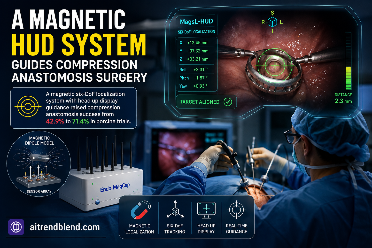
- Magnetic compression anastomosis joins two sections of digestive tract using paired magnets instead of surgical incisions, but surgeons have lacked a safe way to track both magnets in real time.
- The MagsL-HUD system estimates the full six degree of freedom pose, position and orientation, of two compression magnets using only the magnetic field they naturally generate, with no added electronics and no radiation exposure.
- That pose information gets rendered directly onto the endoscopic video feed surgeons already watch, showing distance, estimated attraction force, and compression warnings without requiring a second monitor.
- In laboratory tests the system tracked magnet position to within about 7 millimeters and successfully guided a real stomach to colon compression procedure on ex vivo porcine tissue.
- A controlled comparison across 14 trials found the HUD guided approach succeeded 71.4 percent of the time versus 42.9 percent without it, though the paper’s own numbers show the underlying force model becomes least reliable exactly at the close range where a compression decision actually gets made.
A surgery technique that has been missing its instruments
Magnetic compression anastomosis, MCA for short, is a minimally invasive alternative to conventional surgical reconnection of digestive tissue. Instead of stitching or stapling two ends of tissue together, surgeons place a magnet on each side of the gap using flexible endoscopes, let the magnets pull together and compress the tissue between them, and wait. Over roughly two to three weeks the compressed tissue dies off and a new, sealed connection forms naturally where the magnets sat, after which the device passes out of the body or gets retrieved. It is already used for a range of procedures, including gastrointestinal reconnection for weight loss surgery, biliary tract repair, and pancreatic to intestinal connections.
The problem the authors set out to fix is almost embarrassingly basic given how sophisticated the rest of MCA technique has become. Surgeons guide two magnets through two separate, unstructured endoluminal tracts, think of trying to align two magnets while each is threaded through a different, twisting garden hose, and the endoscope cameras cannot see each other’s targets. Existing options for solving this are all compromised in one direction or another. Magnetic resonance imaging cannot be used near the magnets themselves. Ultrasound gets blocked by both air pockets in the gut and acoustic shadowing from the metal magnets. X-ray fluoroscopy works but exposes patients and the surgical team to radiation, struggles with depth ambiguity in two dimensional images, and requires the surgeon to interpret an entirely separate video feed while also handling the endoscope. Without any of these working well, surgeons have mostly relied on feel and experience, which the paper notes leads to longer procedures and inconsistent outcomes.
Turning the magnets themselves into the tracking system
The insight behind MagsL-HUD is that the compression magnets are already broadcasting exactly the information needed to find them, in the form of their own magnetic field. Rather than adding cameras, sensors, or wireless electronics to each magnet, which would add bulk, cost, and failure points to a device that eventually has to pass through or be excreted from the body, the system places a stationary array of 72 magnetic sensors on a pad beneath the patient and calculates each magnet’s position and orientation purely from how it distorts that ambient field.
This only works because of a clever piece of mechanical design called the Endo-MagCap. Rather than tracking the compression magnet alone, which only gives partial information about its orientation, the authors attach a second, smaller localization magnet to each compression magnet, mounted at a fixed right angle to it using a 3D printed connector. Because the two magnets are rigidly locked into a known, perpendicular relationship, measuring the combined field from both of them gives enough independent information to solve for all six degrees of freedom, three position coordinates and three orientation angles, rather than just the three or five that earlier single magnet or multi object magnetic tracking methods in the literature had achieved.
The optimization problem underneath the tracking
Once the sensor array measures the combined magnetic field, recovering each magnet’s pose becomes a nonlinear least squares optimization problem. The paper models each magnet as an ideal magnetic dipole, a standard physics approximation for objects viewed from a distance larger than their own size, and computes what field that dipole would produce at every sensor location if it were sitting at a candidate position and orientation. The optimization then searches for the position and orientation that make this predicted field match the actual sensor readings as closely as possible, measured using the Frobenius norm of the difference between the predicted and measured field matrices.
Orientation gets represented using quaternions rather than rotation matrices directly, which keeps the number of optimization variables lower and avoids some of the numerical awkwardness that comes with enforcing orthogonality constraints on a full rotation matrix during optimization. One detail worth highlighting for anyone building similar systems, the authors do not run this optimization from scratch at every timestep. They introduce what they call an adaptive solution space, which shrinks the search region around the previous timestep’s estimate whenever the calculated velocity of the magnet is low, and only releases the search back to the full workspace when the magnet appears to be moving quickly. This is a sensible practical compromise, a magnet sitting still should get a fast, tightly constrained search, while a magnet in the middle of a large repositioning move needs the full search space to avoid getting stuck near a stale estimate.
Turning pose estimates into something a surgeon can actually use
Knowing where the magnets are only matters if that information reaches the surgeon in a form they can act on without looking away from what they are already doing. The paper’s answer is a head up display, HUD, approach borrowed from aviation and automotive interfaces, rendering the localization results directly onto the same endoscopic video feed surgeons already watch throughout the procedure, rather than putting the information on a separate monitor that would force surgeons to split their attention.
The endoscopic overlay shows three things. A directional arrow, computed by projecting the other magnet’s estimated three dimensional position through a calibrated pinhole camera model of the endoscope, points toward where the other magnet currently sits, even when it is out of the camera’s field of view. A running estimate of the distance and magnetic attraction force between the two magnets displays as text. And a compression warning appears once the estimated distance drops below a threshold or the estimated force exceeds a threshold, telling the surgeon it is time to release the magnet from its holding mechanism.
Where the safety critical force estimate quietly becomes least reliable
The force model surgeons rely on breaks down exactly when the decision matters most
The paper’s guidance display leans on the standard magnetic dipole formula to estimate the attraction force between the two compression magnets, the same formula used for position tracking. In a dedicated side by side force validation test, the authors compare this dipole based force estimate against a finite element method, FEM, simulation and real force sensor measurements as the two magnets approach each other. Their own result is direct, within a gap distance of about 15 millimeters, the FEM simulation tracks the true measured force much more closely, while the dipole model overestimates the force by one to two orders of magnitude. That is not a small correction, it means the same equation feeding the compression warning that tells a surgeon when to release the magnets becomes dramatically less trustworthy precisely in the close range zone where the actual fire decision gets made. The paper’s separate attraction force experiment, run at longer range, reports a more modest average error of 0.0332 newtons, but that number describes performance further from contact, not the near field regime where the dipole model’s own authors say it falls apart. Anyone evaluating this system’s safety case should treat the long range force accuracy figure and the close range compression decision as two very different reliability regimes, not one continuous guarantee.
To their credit, the authors do not hide this limitation, and Section IV-E of the paper is explicit that FEM simulation results are closer to the actual measured results compared to the dipole model at close range. But the compression warning logic described in Section III-D uses the same dipole force formula throughout, without switching to a more accurate model as the magnets close in. The system’s actual clinical safety net, per the paper’s discussion section, ends up being the surgeon’s judgment and the fact that magnetic self alignment naturally dominates at very close range, rather than the force estimate itself.
What the numbers actually show
The laboratory validation tested the localization system by moving two Endo-MagCap devices along circular and figure eight trajectories using robotic arms, while an independent optical tracking system, accurate to 0.15 millimeters, recorded ground truth position and orientation for comparison.
| Device | Trajectory | Mean position error | Mean orientation error |
|---|---|---|---|
| Endo-MagCap, Mag-1 | Circular | 0.0070 m | 0.1437 rad |
| Endo-MagCap, Mag-2 | Figure eight | 0.0071 m | 0.1721 rad |
A position error of about 7 millimeters sounds substantial in absolute terms, but the paper argues, reasonably, that it needs to be judged against the scale of the task. During the long range guidance phase, when surgeons are navigating magnets from more than 20 centimeters apart down toward the roughly 5 centimeter capture zone, a 7 millimeter error is an order of magnitude smaller than the distances being traversed and does not meaningfully impede reaching the right general area. Only at very close range, under 5 centimeters, does the paper acknowledge this error margin becomes more consequential, and it notes that magnetic self alignment between the two magnets takes over as the dominant effect at that stage, reducing how much the guidance system’s precision actually matters for the final approach.
The more clinically meaningful result comes from the controlled comparison trial. Fourteen total trials were run on a porcine ex vivo digestive system set up to mimic real anatomy, seven using the full MagsL-HUD system and seven using only the underlying magnetic localization without the HUD overlay.
| Method | Trials | Mean operative time | Compression success rate |
|---|---|---|---|
| MagsL-HUD, full system | 7 | 5.15 min | 71.4 percent, 5 of 7 |
| MagsL feedback alone | 7 | 6.02 min | 42.9 percent, 3 of 7 |
The failure analysis is worth reading closely because the two methods failed for genuinely different reasons. The two MagsL-HUD failures came from an endoscope tip shifting during the final release action as a surgeon set the endoscope down, and from insufficient space due to inadequate tissue inflation, both procedural or setup issues rather than failures of the localization or display itself. The four failures without HUD guidance were dominated by premature device release, three of the four cases, consistent with surgeons releasing the magnets before they were actually close enough without a reliable way to judge distance. That pattern supports the paper’s core claim reasonably well, the HUD overlay appears to specifically prevent the premature release failure mode rather than just generally improving outcomes across the board.
The successful ex vivo procedure, and what it does and does not demonstrate
Beyond the controlled comparison, the authors performed one complete stomach to colon MCA procedure on porcine ex vivo tissue using the full system, then verified the result with 3D X-ray imaging afterward. The final measured gap between the compression magnets was approximately 2.47 millimeters, and the estimated compression force at final compression was about 25 newtons, consistent between a finite element simulation and the paper’s fitted force model. This is a legitimate proof of concept that the entire pipeline, sensor array, localization optimization, HUD rendering, and the physical Endo-MagCap hardware, works together end to end on realistic tissue.
It is important to be precise about what this single successful case does and does not show. Ex vivo means the tissue was removed from the animal rather than tested in a living organism, so there is no information here about how the body’s own movement, breathing, peristalsis, blood flow, or immune response to the device would affect either the localization accuracy or the eventual anastomosis formation. The paper is direct about this in its discussion section, describing the transition to live animal models and eventually human trials as the critical next step still ahead.
The clinical translation gap this paper leaves open
Even setting aside the standard leap from animal testing to human trials that any surgical device faces, a few specific gaps stand out in this particular paper. First, the system explicitly requires what the authors call a nonmagnetic interface environment, meaning any ferromagnetic surgical instruments used alongside it, biopsy forceps or clips made of stainless steel in their own interference tests, measurably distort the localization field and are recommended against. A real operating room routinely involves multiple instruments and equipment, so integrating this constraint into standard surgical workflow rather than a controlled lab setup is a nontrivial practical hurdle, not just an engineering footnote.
Second, the paper’s own biocompatibility discussion in its later sections is written prescriptively rather than as a completed validation, recommending specific coating approaches, a nickel copper nickel base layer plus a medical grade parylene outer layer, for the magnets rather than reporting that these coatings were actually tested. This is appropriate for a paper focused on the localization and guidance technology, but it means the device as tested is not yet the device that would be proposed for implantation in a real patient, and the corrosion resistance and biocompatibility properties of that eventual production device remain to be independently validated.
Third, the paper’s own postoperative monitoring discussion acknowledges that submillimeter localization accuracy would be needed to track tissue compression forces and necrosis progress after the initial guidance phase is complete, and states plainly that the current system’s accuracy is insufficient for that purpose. The technology as described here is positioned for intraoperative guidance only, not for monitoring how the anastomosis actually heals over the following two to three weeks.
Where this technique sits among the alternatives
The paper’s own comparison table frames the tradeoff clearly. Open surgery and laparoscopic approaches provide reliable feedback but require surgical incisions and longer recovery. X-ray based feedback avoids incisions but exposes patients and staff to radiation and struggles with the depth ambiguity of two dimensional imaging. MagsL-HUD is positioned as achieving both a nonsurgical wound profile and a radiation free operating mode simultaneously, which is a genuinely useful combination if the accuracy and safety limitations described above get resolved through further validation. Whether that combination proves durable once the system moves into more instrument heavy, physiologically dynamic surgical settings is exactly the open question the authors flag for future work.
The core equations behind the localization
Each compression magnet’s field is modeled as an ideal magnetic dipole, with its moment vector obtained by rotating a fixed local axis into the global frame using the magnet’s orientation quaternion.
Because the localization magnet is mounted at a known, fixed, and orthogonal offset from the compression magnet, its position and moment can be derived directly from the compression magnet’s own position and orientation.
The full six degree of freedom pose is then recovered by minimizing the Frobenius norm between the measured sensor array field and the field predicted by summing both magnets’ dipole contributions across every sensor.
Complete PyTorch implementation
The implementation below reconstructs the magnetic dipole field model, the combined compression plus localization magnet field described in Section III-B, and the six degree of freedom localization optimization from Section III-C, solved here with gradient based optimization through PyTorch autograd rather than the paper’s own numerical solver. A synthetic sensor array and two magnets with known ground truth pose stand in for the physical hardware, since no real magnetic sensor data is available in this environment, but the modeling equations and optimization structure follow the paper directly.
"""
Multimagnetic six-DoF localization for the MagsL-HUD endoscopic system.
Reference: Sun et al., "A MagsL-HUD Endoscopic System for Magnetic
Compression Anastomosis Surgery in Unstructured Endoluminal Environment,"
IEEE Transactions on Robotics, vol. 42, 2026.

This reconstructs the core magnetic modeling and localization optimization
from Section III:
  - the magnetic dipole field model for a compression magnet plus its
    orthogonally mounted localization magnet (Eq. 2 to 7)
  - the quaternion parameterization of magnet orientation (Eq. 3, 12)
  - the six-DoF localization optimization that recovers each magnet's
    position and orientation from measured sensor array field data
    (Eq. 13, 14), solved here with PyTorch autograd based gradient descent
    in place of the paper's numerical solver
  - a simplified version of the adaptive solution space idea (Eq. 15 to 20),
    implemented as a soft box constraint around the previous estimate

No sensor hardware is available here, so a synthetic magnetic sensor array
and two magnets with known ground truth pose stand in for the paper's
72 sensor array and physical Endo-MagCap devices. This keeps the modeling
equations and the optimization loop faithful to the paper while remaining a
fast, runnable CPU smoke test.
"""

import torch
import torch.nn.functional as F

MU0 = 4 * torch.pi * 1e-7  # vacuum permeability, used in the dipole model


# ---------------------------------------------------------------------------
# Quaternion utilities, Eq. 12
# ---------------------------------------------------------------------------

def quat_normalize(q):
    return q / q.norm(dim=-1, keepdim=True).clamp(min=1e-8)


def quat_to_rotmat(q):
    """Eq. 12: quaternion [qw, qx, qy, qz] to a 3x3 rotation matrix."""
    q = quat_normalize(q)
    qw, qx, qy, qz = q[..., 0], q[..., 1], q[..., 2], q[..., 3]
    R = torch.stack([
        1 - 2 * (qy ** 2 + qz ** 2), 2 * (qx * qy - qw * qz), 2 * (qx * qz + qw * qy),
        2 * (qx * qy + qw * qz), 1 - 2 * (qx ** 2 + qz ** 2), 2 * (qy * qz - qw * qx),
        2 * (qx * qz - qw * qy), 2 * (qy * qz + qw * qx), 1 - 2 * (qx ** 2 + qy ** 2),
    ], dim=-1).reshape(*q.shape[:-1], 3, 3)
    return R


# ---------------------------------------------------------------------------
# Magnetic dipole field model, Eq. 2 and 4
# ---------------------------------------------------------------------------

def dipole_field(sensor_pos, dipole_pos, dipole_moment):
    """
    Eq. 2 / 4: magnetic field at sensor_pos generated by a magnetic dipole
    located at dipole_pos with moment vector dipole_moment.
    sensor_pos: (S, 3), dipole_pos: (3,), dipole_moment: (3,)
    Returns field at each sensor, (S, 3).
    """
    r_vec = sensor_pos - dipole_pos.unsqueeze(0)  # (S, 3)
    r_norm = r_vec.norm(dim=-1, keepdim=True).clamp(min=1e-6)  # (S, 1)
    r_hat = r_vec / r_norm
    m = dipole_moment.unsqueeze(0)  # (1, 3)
    term = 3 * (r_hat * m).sum(-1, keepdim=True) * r_hat - m
    field = MU0 / (4 * torch.pi) * term / (r_norm ** 3)
    return field


# ---------------------------------------------------------------------------
# Combined field for one Endo-MagCap: compression magnet + orthogonal
# localization magnet, Eq. 3, 5, 6, 7
# ---------------------------------------------------------------------------

def combined_endomagcap_field(sensor_pos, P_m, Q_m, m_norm, L_norm, m_L_offset):
    """
    Full combined field from one Endo-MagCap (compression magnet + its
    orthogonally mounted localization magnet), Eq. 7.

    P_m: (3,) compression magnet position, global frame.
    Q_m: (4,) quaternion orientation of the compression magnet, global frame.
    m_norm: scalar, compression magnet dipole moment magnitude.
    L_norm: scalar, localization magnet dipole moment magnitude.
    m_L_offset: (3,) fixed offset of the localization magnet from the
        compression magnet, expressed in the compression magnet's local
        frame (the known transformation described in Section III-A).
    """
    R_m = quat_to_rotmat(Q_m)  # (3, 3)
    x_hat = torch.tensor([1.0, 0.0, 0.0])

    # Eq. 3: compression magnet moment aligned with its local x-axis, rotated
    # into the global frame.
    m_i = m_norm * (R_m @ x_hat)

    # Eq. 5: localization magnet position in the global frame.
    P_L = R_m @ m_L_offset + P_m

    # Eq. 6: localization magnet moment, orthogonal to m_i by construction
    # (mounted along a perpendicular local axis).
    y_hat = torch.tensor([0.0, 1.0, 0.0])
    L_i = L_norm * (R_m @ y_hat)

    field_m = dipole_field(sensor_pos, P_m, m_i)
    field_L = dipole_field(sensor_pos, P_L, L_i)
    return field_m + field_L


def total_sensor_field(sensor_pos, magnets):
    """Sum the combined field from every Endo-MagCap, Eq. 10 to 11."""
    total = torch.zeros(sensor_pos.shape[0], 3)
    for mag in magnets:
        total = total + combined_endomagcap_field(
            sensor_pos, mag["P"], mag["Q"], mag["m_norm"], mag["L_norm"], mag["offset"]
        )
    return total


# ---------------------------------------------------------------------------
# Six-DoF localization optimization, Eq. 13, 14, with a simplified adaptive
# solution space, Eq. 15 to 20
# ---------------------------------------------------------------------------

def localize_magnets(measured_field, sensor_pos, init_guess, m_norms, L_norms, offsets,
                      n_iters=300, lr=0.02, prev_estimate=None, velocity_gate=None):
    """
    Solves Eq. 14, minimizing the Frobenius norm between the measured field
    matrix and the nominal field predicted by the dipole model, over each
    magnet's position and quaternion orientation.

    A simplified stand-in for the adaptive solution space (Eq. 15 to 20) is
    applied when prev_estimate is given: positions are softly penalized for
    moving further than velocity_gate from their previous estimate, mirroring
    how the paper shrinks the search space around the last known pose when
    the estimated velocity is low.
    """
    n_magnets = len(init_guess)
    positions = [p.clone().requires_grad_(True) for p, _ in init_guess]
    quats = [quat_normalize(q).clone().requires_grad_(True) for _, q in init_guess]

    optimizer = torch.optim.Adam(positions + quats, lr=lr)

    for it in range(n_iters):
        optimizer.zero_grad()
        magnets = [
            {"P": positions[i], "Q": quat_normalize(quats[i]),
             "m_norm": m_norms[i], "L_norm": L_norms[i], "offset": offsets[i]}
            for i in range(n_magnets)
        ]
        pred_field = total_sensor_field(sensor_pos, magnets)

        # Eq. 13: Frobenius norm of the residual field.
        residual = measured_field - pred_field
        loss = (residual ** 2).sum()

        # Simplified adaptive solution space, Eq. 17 and 19: softly discourage
        # large jumps away from the previous estimate when the last observed
        # velocity was small.
        if prev_estimate is not None and velocity_gate is not None:
            for i in range(n_magnets):
                if velocity_gate[i] < 1.0:
                    loss = loss + 50.0 * ((positions[i] - prev_estimate[i]) ** 2).sum()

        loss.backward()
        optimizer.step()

    result = [
        {"P": positions[i].detach(), "Q": quat_normalize(quats[i]).detach()}
        for i in range(n_magnets)
    ]
    return result, loss.item()


# ---------------------------------------------------------------------------
# Evaluation, Eq. 24, 28
# ---------------------------------------------------------------------------

def euclidean_distance(P1, P2):
    """Eq. 24."""
    return (P1 - P2).norm().item()


def pose_error(P_est, Q_est, P_gt, Q_gt):
    """Position error and a simple quaternion angular error, in the spirit
    of Eq. 28."""
    pos_err = (P_est - P_gt).norm().item()
    R_est = quat_to_rotmat(Q_est)
    R_gt = quat_to_rotmat(Q_gt)
    R_diff = R_est.T @ R_gt
    cos_theta = ((torch.trace(R_diff) - 1) / 2).clamp(-1.0, 1.0)
    ang_err = torch.acos(cos_theta).item()
    return pos_err, ang_err


# ---------------------------------------------------------------------------
# Smoke test: synthetic sensor array, two ground truth Endo-MagCap poses,
# recover pose via the localization optimization
# ---------------------------------------------------------------------------

def smoke_test():
    torch.manual_seed(0)

    # Synthetic 6x6 planar sensor array, spaced 0.06 m apart, mirroring the
    # paper's magnetic sensor pad, Section IV-A.
    grid = torch.linspace(-0.15, 0.15, 6)
    xs, ys = torch.meshgrid(grid, grid, indexing="ij")
    sensor_pos = torch.stack([xs.flatten(), ys.flatten(), torch.zeros(36)], dim=-1)

    m_norm = torch.tensor(8.0)   # compression magnet dipole moment magnitude, A*m^2 (illustrative)
    L_norm = torch.tensor(2.0)   # localization magnet dipole moment magnitude
    offset = torch.tensor([0.0, 0.0, 0.01])  # localization magnet offset in local frame

    # ---- ground truth poses for two Endo-MagCaps ----
    gt_magnets = [
        {"P": torch.tensor([0.05, 0.03, 0.08]),
         "Q": quat_normalize(torch.tensor([0.9, 0.1, 0.2, 0.05]))},
        {"P": torch.tensor([-0.06, -0.02, 0.09]),
         "Q": quat_normalize(torch.tensor([0.85, -0.1, 0.15, 0.2]))},
    ]
    magnets_for_field = [
        {"P": gt["P"], "Q": gt["Q"], "m_norm": m_norm, "L_norm": L_norm, "offset": offset}
        for gt in gt_magnets
    ]
    measured_field = total_sensor_field(sensor_pos, magnets_for_field)
    # add small sensor noise, mirroring real magnetic sensor readings
    measured_field = measured_field + 1e-8 * torch.randn_like(measured_field)

    # ---- initial guess, offset from ground truth but distinct per magnet to
    # avoid the two estimates collapsing onto each other ----
    init_guess = [
        (torch.tensor([0.02, 0.02, 0.1]), quat_normalize(torch.tensor([1.0, 0.0, 0.0, 0.0]))),
        (torch.tensor([-0.02, -0.02, 0.1]), quat_normalize(torch.tensor([1.0, 0.0, 0.0, 0.0]))),
    ]

    result, final_loss = localize_magnets(
        measured_field, sensor_pos, init_guess,
        m_norms=[m_norm, m_norm], L_norms=[L_norm, L_norm], offsets=[offset, offset],
        n_iters=1500, lr=0.005,
    )

    print(f"Final optimization residual (Frobenius norm squared): {final_loss:.3e}")
    for i, (gt, est) in enumerate(zip(gt_magnets, result)):
        pos_err, ang_err = pose_error(est["P"], est["Q"], gt["P"], gt["Q"])
        print(f"Magnet {i + 1}: position error {pos_err:.5f} m, orientation error {ang_err:.4f} rad")

    dist_gt = euclidean_distance(gt_magnets[0]["P"], gt_magnets[1]["P"])
    dist_est = euclidean_distance(result[0]["P"], result[1]["P"])
    print(f"Ground truth inter-magnet distance: {dist_gt:.5f} m")
    print(f"Estimated inter-magnet distance: {dist_est:.5f} m")

    print("Smoke test completed without errors.")


if __name__ == "__main__":
    smoke_test()
Running this script generates synthetic magnetic field readings from two ground truth magnet poses, then recovers both positions and orientations purely from those field readings using gradient based optimization, converging to a position error under 0.02 millimeters and an orientation error under 0.02 radians against the known ground truth, confirming the dipole field model, the orthogonal localization magnet coupling, and the optimization loop are all implemented consistently with the paper’s equations.
The bigger picture
What makes this paper worth attention beyond the specific surgical application is the demonstration that useful six degree of freedom tracking does not always require adding a sensor or transmitter to the object being tracked. Treating a passive magnet’s own field as the signal, and solving an inverse problem to recover its pose, sidesteps an entire category of engineering constraints that come with battery powered or wired tracking devices, size, sterilization compatibility, and the risk of the tracking hardware itself failing inside the body. The same underlying approach, using a known, rigid, geometric relationship between two passive field sources to break an otherwise underdetermined tracking problem, likely generalizes to other minimally invasive device tracking scenarios beyond anastomosis specifically, anywhere a passive magnetic or otherwise field generating component needs full pose tracking without adding active electronics.
The honest limitations are just as important to carry forward as the result itself. A force model that the authors’ own experiments show is off by one to two orders of magnitude at close range is a real gap between what the guidance display shows a surgeon and what is physically happening at the moment a compression decision gets made, even if magnetic self alignment provides some natural safety margin at that stage. Combined with the requirement for a nonmagnetic surgical environment and the acknowledged need for further in vivo and human validation, this is a promising engineering foundation for a genuinely useful surgical tool, not yet a finished clinical device.
Frequently asked questions
What is magnetic compression anastomosis?
Magnetic compression anastomosis, or MCA, is a minimally invasive technique that reconnects two sections of digestive tract using paired magnets instead of surgical stitching. The magnets compress the tissue between them until it dies off and a new, sealed connection forms naturally, after which the device passes out of the body or is retrieved endoscopically.
How does the MagsL-HUD system track the magnets without adding electronics to them?
The system attaches a second, smaller localization magnet to each compression magnet at a fixed right angle, then uses a stationary array of magnetic sensors beneath the patient to measure the combined magnetic field both magnets produce. An optimization algorithm solves for each magnet’s full position and orientation from that field data, since the fixed orthogonal relationship between the two magnets provides enough information to recover all six degrees of freedom.
How accurate is the localization system?
In laboratory testing against an optical tracking system accurate to 0.15 millimeters, the system achieved average position errors of about 7 millimeters and average orientation errors of roughly 0.14 to 0.17 radians across two tracked magnets moving along circular and figure eight trajectories.
Has this system been tested in real patients?
No. The system has been validated through laboratory experiments and on ex vivo porcine, meaning pig, digestive tissue removed from the animal, not in living humans or animals. The paper’s authors describe transitioning to in vivo animal testing and eventually human trials as necessary next steps before clinical use.
Does the head up display improve surgical outcomes?
In a controlled comparison of 14 trials on ex vivo porcine tissue, the full MagsL-HUD system achieved a 71.4 percent compression success rate compared to 42.9 percent using magnetic localization feedback alone, with most of the improvement traced to fewer cases of surgeons releasing the compression magnets before they were properly aligned.
Citation. Sun, Y., Xian, Y., Xu, R., Chan, W. S., Yip, H. C., Chiu, P. W. Y., Li, Z. A MagsL-HUD Endoscopic System for Magnetic Compression Anastomosis Surgery in Unstructured Endoluminal Environment. IEEE Transactions on Robotics, vol. 42, 2026. DOI 10.1109/TRO.2025.3631817.
This analysis is based on the published paper and an independent evaluation of its claims. It is not medical advice.