
Important context before you read further
The source document behind this article is a graduate course project report from Columbia University’s ECS E6692, Deep Learning on the Edge, not a peer reviewed clinical study, and it has not been evaluated by a medical regulatory body. It builds on a real peer reviewed method, a 2022 cross-architecture knowledge distillation paper, and applies it to a new domain as a class assignment.
Nothing in this article should be read as evidence that the described system is validated, approved, or ready for real world disease screening. We report the paper’s own numbers, including places where those numbers are internally inconsistent or where the authors themselves flag a bug in their results, because that context matters for understanding what the project actually demonstrated. This article is about the distillation technique, not a medical recommendation, and it is not a substitute for advice from an eye care professional.
Key points
- The project distills a Vision Transformer teacher, pretrained with I-JEPA self-supervised learning, into a much smaller CNN student for four class retinal disease classification.
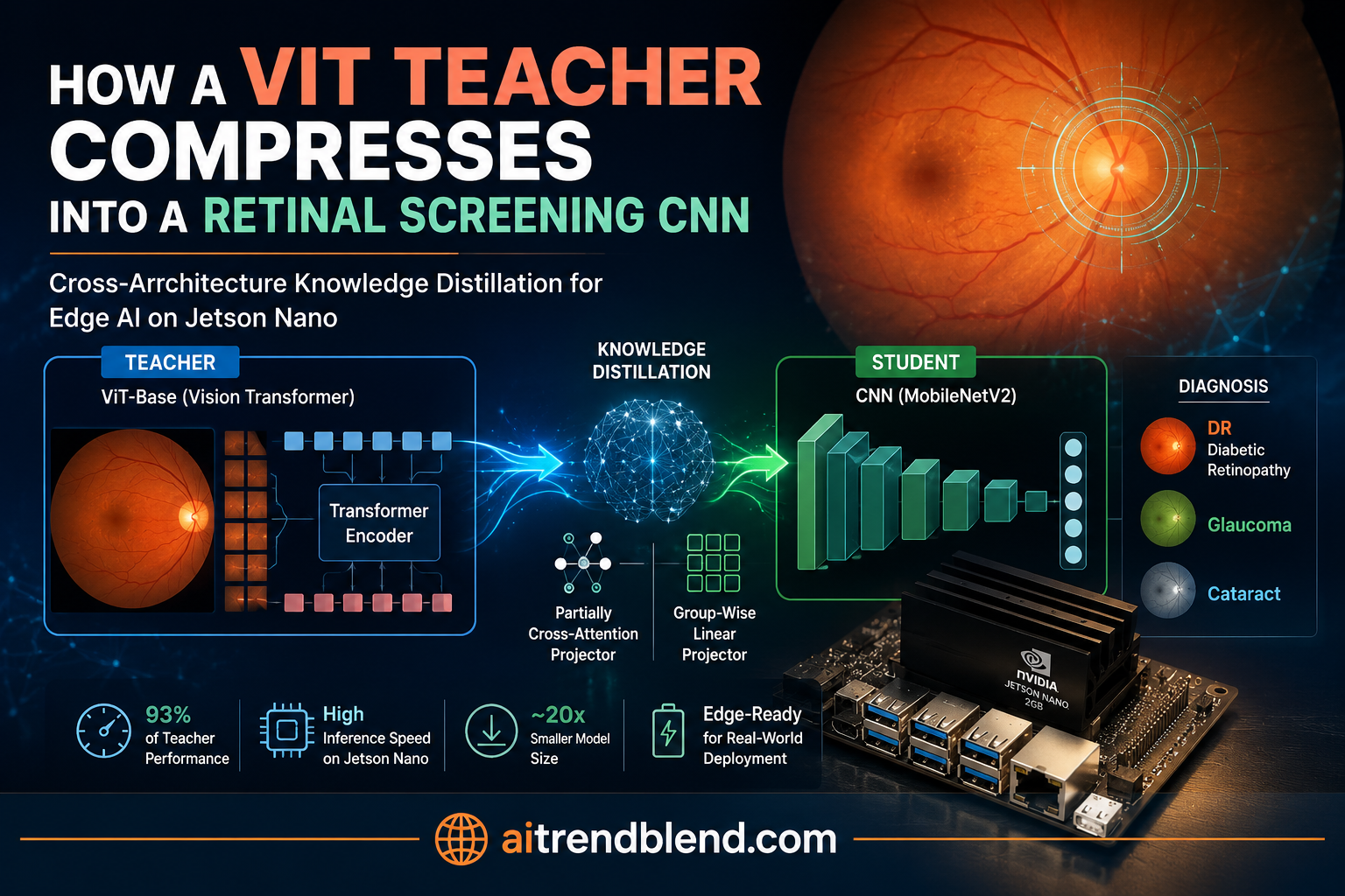
- Cross-architecture distillation is harder than same-architecture distillation because CNN feature maps and transformer patch embeddings are structured completely differently, so the project uses two custom projectors to bridge that gap.
- A Partially Cross-Attention projector teaches the CNN to mimic the transformer’s self-attention patterns, while a Group-Wise Linear projector aligns the two models’ feature spaces directly.
- The compressed student model has 2,228,996 parameters against the teacher’s 85,801,732, a 97.4 percent reduction, and reportedly retains about 93 percent of the teacher’s diagnostic performance.
- Without knowledge distillation, the same small CNN trained from scratch performs close to randomly, with an F1 score of just 0.04 on the majority Normal class, underscoring how much of the reported gain comes from the distillation process itself rather than the architecture choice.
- The report is transparent about its own rough edges, including a small and imbalanced dataset, a shortened fifty epoch training run, and a self-acknowledged bug where a claimed quantization step does not appear to have actually reduced the model’s file size.
Why a good retinal classifier still might not reach the clinic that needs it
Diabetic retinopathy, glaucoma, and cataracts are all detectable through a retinal fundus photograph, and deep learning models, particularly vision transformers, have gotten very good at spotting the patterns that indicate each one. The trouble is that being accurate and being deployable are two different problems. A vision transformer capable enough to classify these conditions reliably tends to carry tens of millions of parameters, memory demands that exceed what a low cost edge device can hold, and inference latency too slow to be useful in a real clinical workflow. That combination puts this class of model out of reach for exactly the settings where it could matter most, primary care locations without a specialist ophthalmologist on site and without server grade computing hardware.
The project’s proposed fix is knowledge distillation, training a small student model to imitate a large teacher model’s behavior, paired with a specific architectural twist. Rather than distilling a large transformer into a smaller transformer, which is the more common and more straightforward setup, the authors distill into a convolutional neural network instead, chosen because CNNs are generally cheaper to run on constrained edge hardware than transformers are, even at a comparable parameter count. That choice is what makes the project technically interesting and also what makes it hard, since CNNs and transformers do not represent visual information the same way at all.
Why teacher and student speak different visual languages
A convolutional network builds up its understanding of an image through local filters sliding across the pixel grid, producing feature maps organized by spatial position and channel. A vision transformer instead slices the image into a grid of patches, treats each patch like a token in a sentence, and lets every patch attend to every other patch through self-attention, producing a very different kind of representation, one built around long range relationships between distant regions rather than local neighborhoods. The paper argues this distinction matters clinically, not just architecturally, because subtle pathological patterns in a retina can depend on the relationship between distant regions of the same image, exactly the kind of global context that self-attention captures well and that a purely local CNN filter can miss.
Standard knowledge distillation, the version introduced by Hinton and colleagues in 2015, was built with same-architecture transfer in mind and mostly works by having the student match the teacher’s softened output probabilities.
That works fine when teacher and student share a similar internal structure, but it leaves a real gap when the student’s internal features have no direct counterpart in the teacher’s internal features, exactly the situation a CNN student and a transformer teacher create. The project addresses that gap with two purpose built projector modules, discussed below, both adapted from a 2022 paper on cross-architecture knowledge distillation that the authors cite as their foundation.
Takeaway
The core engineering problem here is not compression itself, which knowledge distillation already handles reasonably well, it is translation, finding a way for a model that thinks in local convolutional filters to meaningfully absorb knowledge from a model that thinks in global self-attention.
Building a teacher worth compressing
Before any distillation can happen, the project needs a strong teacher model, and getting there involves a two stage process, self-supervised pretraining followed by supervised fine tuning.
Pretraining with I-JEPA, learning from unlabeled retinas
Labeled medical images are expensive to produce, since they require an expert to review and annotate each one, while unlabeled images are comparatively easy to collect. The project’s teacher model starts with I-JEPA, a self-supervised learning method that sits between two more familiar approaches, contrastive learning and pixel level reconstruction. Contrastive methods like SimCLR rely on data augmentations that risk distorting clinically meaningful features in a medical image. Reconstruction based methods like masked autoencoders focus heavily on pixel level detail rather than higher level semantic understanding. I-JEPA instead predicts masked regions of an image directly in a learned representation space, encouraging the model to capture meaningful patterns rather than surface level texture.
A context encoder processes the visible parts of an image, a target encoder builds representations of the masked parts, and a predictor network tries to guess the target representations from the context alone, using a block-wise masking strategy that hides sixty to seventy five percent of the image at once, forcing the model to reason about large missing regions rather than filling in small gaps. The target encoder’s parameters update through an exponential moving average of the context encoder rather than direct gradient descent, a stabilizing trick borrowed from earlier self-supervised methods.
The project reports this pretraining stage running for 20 epochs, with the training loss dropping from 3.18 to 2.60, followed by 15 epochs of supervised fine tuning where training accuracy passed 90 percent by epoch 3 and validation accuracy peaked at 91.49 percent by epoch 14. The final teacher, built on a ViT-Base architecture with roughly 85.8 million parameters, reached 92.87 percent accuracy on the held out test set across the four diagnostic categories.
The two projectors that bridge the architectural gap
With a capable teacher in hand, the real technical contribution of the project is the pair of projector modules that let a CNN student learn from that transformer teacher despite their structurally different feature representations.
The Partially Cross-Attention projector, teaching a CNN to pay transformer-style attention
The Partially Cross-Attention projector, shortened to PCA in the paper, gives the CNN student a mechanism for mimicking the teacher’s self-attention behavior. Three parallel convolutional layers project the student’s CNN feature map into query, key, and value representations, the same three components self-attention is built from in a transformer.
From there, the student computes its own attention map using the same scaled dot product formula a transformer uses internally.
The teacher’s own genuine self-attention map, taken directly from its transformer layers, then acts as a target the student’s synthetic attention map is trained to match, using KL divergence between the two attention distributions.
The intuition is straightforward once you see the mechanics, rather than trying to force the CNN’s local convolutional filters to somehow become transformer layers, this projector gives the CNN a lightweight, learnable stand in for self-attention that gets explicitly trained to reproduce the teacher’s attention pattern, letting the student pick up on the kind of long range, cross-region relationships in a retina that a plain CNN would otherwise have no mechanism for capturing at all.
The Group-Wise Linear projector, reconciling two different feature spaces
Even with an attention mimicking mechanism in place, the CNN’s raw feature representations and the transformer’s patch embeddings still live in fundamentally different formats, a CNN feature map structured as channels by spatial resolution against a transformer’s patches by flattened embedding dimension. The Group-Wise Linear projector, shortened to GL, handles this second alignment problem by splitting the CNN’s feature channels into groups and applying a separate learnable linear transformation to each group before concatenating the results back together.
The resulting projected features are then trained to match the teacher’s corresponding features directly, using a simple mean squared error loss.
Splitting the transformation into groups rather than using one enormous linear layer keeps the parameter count of this projector comparatively small, which matters given the whole point of the project is to end up with something deployable on constrained hardware in the first place.
Multi-view training and an adversarial nudge toward realistic generalization
The final piece is a multi-view training scheme meant to make the distilled student more robust to the kind of variation real clinical images actually show, different cameras, different lighting, different framing. For each training image, the project generates several additional augmented views through cropping and other transformations, and trains the distillation losses across all of these views rather than a single fixed image each time.
On top of that, a small discriminator network tries to tell apart the teacher’s real features from the student’s projected features, while the student is trained to fool it, an adversarial setup borrowed from generative adversarial network training rather than a direct feature matching objective.
Worth flagging directly, the paper’s own methodology section combines these three losses into a total objective written as \( L_{Total} = L_{PCA} + \lambda_1 L_{GL} + \lambda_2 L_{adv} \), while the implementation section later describes the same combination in slightly different terms as PCA loss plus a weighted GL loss plus an unweighted robust loss. The two descriptions are not word for word consistent with each other, a small but real internal inconsistency worth knowing about if you go looking at the underlying formulas closely, or if you attempt to reproduce the exact weighting scheme from the paper text alone rather than from the authors’ published code.
The dataset, and the imbalance that shaped everything downstream
The project trained and evaluated on 6,727 retinal fundus images split into four diagnostic categories, Normal, Diabetic Retinopathy, Glaucoma, and Cataract, divided into 4,997 training images, 1,057 validation images, and 673 test images. The training set carries a real class imbalance that the authors describe as reflecting actual clinical prevalence, Normal cases making up 38.5 percent of the training data, Diabetic Retinopathy 29.9 percent, Glaucoma 17.6 percent, and Cataract only 14.0 percent. To address this, the project applied class weighting during training along with condition specific data augmentation, using more aggressive augmentation for the underrepresented Cataract and Glaucoma classes, and tailoring the specific augmentation type to each condition, for example limiting rotation for Glaucoma cases specifically to avoid distorting the optic cup and disc features that matter for that diagnosis.
It is worth being upfront that 6,727 total images is a small dataset by general computer vision standards, and the authors say as much themselves, attributing the small size to the general scarcity of available medical imaging data compared to natural image benchmarks. That scarcity is a genuine, well known constraint across medical imaging research broadly, not something specific to this project, but it does mean the reported performance numbers come from a comparatively narrow evidence base.
Does the distilled student actually hold up
The results section is where the project’s real payoff shows up, and also where its most useful caveats live. Two student models get compared, one trained the ordinary way directly on the labeled dataset with no distillation at all, and one trained using the full cross-architecture distillation pipeline.
Without distillation, the small CNN barely functions
Trained from scratch on its own, without any signal from the teacher, the small CNN student performs close to randomly. Its precision, recall, and F1 scores per class tell a stark story.
| Class, base student without KD | Precision | Recall | F1 | Support |
|---|---|---|---|---|
| Cataract | 0.14 | 0.33 | 0.20 | 104 |
| Diabetic Retinopathy | 0.30 | 0.22 | 0.25 | 167 |
| Glaucoma | 0.19 | 0.42 | 0.26 | 131 |
| Normal | 0.26 | 0.02 | 0.04 | 271 |
| Macro average | 0.22 | 0.25 | 0.19 | 673 |
The Normal class, despite being the largest single category in the dataset by a wide margin, gets an F1 score of just 0.04, meaning the undistilled model essentially fails to recognize the most common class correctly in almost every case. The paper reports the corresponding ROC curves sit close to the diagonal line, with AUC values around 0.50, which is the statistical signature of a classifier with no real discriminative ability at all, no better than flipping a coin.
With distillation, the same architecture becomes genuinely useful
The identical CNN architecture, trained instead through the full cross-architecture distillation pipeline for 50 epochs, looks like a different model entirely.
| Class, distilled student with KD | Precision | Recall | F1 | Support |
|---|---|---|---|---|
| Cataract | 0.95 | 0.86 | 0.90 | 104 |
| Diabetic Retinopathy | 0.97 | 0.92 | 0.94 | 167 |
| Glaucoma | 0.84 | 0.69 | 0.76 | 131 |
| Normal | 0.84 | 0.97 | 0.90 | 271 |
| Macro average | 0.90 | 0.86 | 0.88 | 673 |
Every metric across every class improved substantially, and the reported ROC AUC values climb to between 0.96 and 0.99 across all four categories. The paper describes the overall global accuracy of the distilled student as 89 percent during training monitoring, and separately reports the best validation checkpoint reaching 87.0 percent at epoch 40, described as 93.8 percent of the teacher’s 92.87 percent test accuracy. Glaucoma stands out as the weakest performing class throughout, with a recall of 0.69 in the final distilled model, and the confusion matrix shows a specific, clinically relevant confusion pattern, fourteen Cataract images misclassified as Glaucoma and thirty six Glaucoma images misclassified as Normal, the latter being a more concerning kind of error in a real screening context since it means missing an actual case of a sight threatening condition.
The significant performance gap between the non-distilled baseline student, at 20 percent accuracy, and the distilled student, at 89 percent, highlights the critical role of the projection methods in narrowing the architectural gap between transformers and CNNs.Reading of the project’s own discussion section
A numbers mismatch worth flagging directly
Reporting inconsistency in the source document
Section 5.1.2 of the report states the distilled student achieved 97.4 percent accuracy on Normal cases and 91.6 percent on Diabetic Retinopathy. A few pages later, Section 5.1.3 directly compares teacher and student accuracy per class and instead reports the student at 81 percent on Normal and 82 percent on DR, against a teacher at 88 percent and 89 percent respectively for those same two classes. Those two sets of numbers, for what should be the same trained model, do not match each other, and the report does not explain the discrepancy. It’s possible these come from different evaluation runs, different checkpoints, or a transcription error somewhere in the writing process, but as published the numbers are simply inconsistent with each other. We report both sets here rather than picking one to feature, since presenting only the more favorable figures would misrepresent how settled this project’s results actually are.
Shrinking the model, and an honestly reported bug
The headline compression numbers are clean and easy to verify against each other. The teacher model carries 85,801,732 parameters, the student carries 2,228,996, a reduction of 97.4 percent, landing at a final model size of 8.79 megabytes, comfortably within the memory budget of a Jetson Nano 2GB device. Framed against the reported 93 percent performance retention, that is a genuinely favorable tradeoff on paper, shedding the overwhelming majority of the parameter count while keeping most of the diagnostic behavior.
Where the report deserves real credit is in how it handles a problem in its own deployment pipeline. The authors attempted a further quantization step on the already compressed student model and report comparing accuracy and throughput between the plain student CNN and the quantized version on the actual Jetson Nano hardware. Reported throughput more than doubled, from 2.19 images per second to 5.41 images per second, which would ordinarily be presented as a clean quantization win. Instead, the authors include a direct note flagging that the model file sizes before and after quantization were identical, meaning the quantization step likely did not save correctly, and they attribute the observed throughput increase to the GPU warming up between runs rather than to any actual effect of quantization. They add that the accuracy metrics and confusion matrices from that stage remain accurate even though the quantization claim itself does not hold up. That kind of self-reported negative result is unusual to see included rather than quietly dropped, and it is a genuinely useful signal about how much further validation this specific pipeline would need before treating its edge deployment numbers as settled.
What the discussion section gets right about its own limits
To its credit, the report’s discussion section does not oversell its results. The authors are direct that their dataset is small relative to typical computer vision benchmarks due to the general scarcity of available medical imaging data, that they trained for only 50 epochs against the 100 or more epochs used in comparable prior work due to computational and time constraints, and that while the underlying distillation framework supports several CNN student architectures, including MobileNetV2, ResNet18, EfficientNet-B0, and SqueezeNet1.1, they narrowed their own experiments to a single optimized architecture in order to focus specifically on the Jetson Nano deployment target rather than conducting a broader architecture comparison.
The authors also offer a plausible explanation for why performance varies so much across the four diagnostic classes, with Normal and Diabetic Retinopathy classified far more reliably than Glaucoma. Normal images, they reason, likely have a more visually consistent appearance with clearer anatomical structure and no pathological changes to complicate classification, and Normal cases also made up the largest share of the training data by a wide margin, giving the model simply more examples to learn from for that class specifically. The observed confusion between Cataract and Glaucoma, meanwhile, is attributed to the two conditions sharing overlapping visual characteristics in a fundus photograph, a reasonable hypothesis though one the report does not test directly with any further analysis.
Honest limitations
This is an unreviewed graduate course project report, not a peer reviewed publication, and its numbers have not been independently verified or replicated by anyone outside the two student authors and their course instructors.
Internal inconsistencies exist within the report itself, most notably the mismatched per class accuracy figures between Section 5.1.2 and Section 5.1.3 discussed above, which means the headline performance retention figure should be treated as an approximate, self-reported estimate rather than a precise, independently confirmed number.
The dataset of 6,727 images is small, and the authors’ own explanation for class-by-class performance differences, tied partly to how much training data each class had, suggests results could shift meaningfully with a larger or differently balanced dataset.
Training ran for only 50 epochs due to stated computational and time constraints, short of the 100 or more epochs the authors note comparable prior work has used, leaving open whether extended training would change the reported numbers.
The quantization step, one of the two edge optimization techniques evaluated for Jetson Nano deployment, is explicitly flagged by the authors as not having worked as intended, with the reported throughput improvement attributed to GPU warmup rather than to the compression technique itself.
The framework was evaluated against only a single CNN student architecture in the reported experiments, despite the underlying code supporting several, so it remains unclear how sensitive the results are to that specific architecture choice.
Where this fits in the wider model compression picture
Set the medical framing aside for a moment and the underlying engineering idea generalizes well past retinal imaging specifically. Any setting that wants to deploy a transformer’s accuracy on hardware that can only realistically run a CNN, industrial visual inspection on embedded cameras, wildlife camera traps in the field, or any other computer vision task constrained to genuinely cheap edge hardware, faces the same architectural mismatch problem this project tackles. The general recipe demonstrated here, an attention mimicking projector paired with a feature space alignment projector and a multi-view adversarial training scheme, is a reasonable template to test in any of those adjacent cross-architecture compression settings, independent of whether the downstream task happens to be medical.
Complete PyTorch implementation
The project’s own code is publicly available on GitHub, linked in the footnote below. For a compact, self-contained illustration of the core mechanics, here is an independent reimplementation covering the Partially Cross-Attention projector, the Group-Wise Linear projector, a simplified multi-view generator, a small adversarial discriminator, the combined loss, a training step with a frozen teacher, and a smoke test on randomly generated dummy image batches.
# cross_architecture_kd_reimplementation.py
# Independent PyTorch reimplementation of the cross-architecture knowledge
# distillation pipeline described in a Columbia University E6692 course
# project applying Liu et al.'s 2022 Cross-Architecture Knowledge
# Distillation method to retinal fundus classification. This is not the
# original authors' code, it is a reconstruction built from the report's
# equations for educational use. Their own implementation is linked below.

import torch
import torch.nn as nn
import torch.nn.functional as F


class PCAProjector(nn.Module):
    # Partially Cross-Attention projector, gives a CNN feature map a
    # transformer-style self-attention mechanism to mimic the teacher's attention.
    def __init__(self, channels):
        super().__init__()
        self.q_proj = nn.Conv2d(channels, channels, kernel_size=1)
        self.k_proj = nn.Conv2d(channels, channels, kernel_size=1)
        self.v_proj = nn.Conv2d(channels, channels, kernel_size=1)
        self.channels = channels

    def forward(self, feat):
        b, c, h, w = feat.shape
        q = self.q_proj(feat).view(b, c, h * w).permute(0, 2, 1)  # [b, hw, c]
        k = self.k_proj(feat).view(b, c, h * w)  # [b, c, hw]
        v = self.v_proj(feat).view(b, c, h * w).permute(0, 2, 1)  # [b, hw, c]

        attn_scores = torch.bmm(q, k) / (self.channels ** 0.5)  # [b, hw, hw]
        attn_map = F.softmax(attn_scores, dim=-1)

        context = torch.bmm(attn_map, v)  # [b, hw, c]
        context = context.permute(0, 2, 1).view(b, c, h, w)
        return context, attn_map


def pca_loss(student_attn, teacher_attn, eps=1e-8):
    # KL divergence between teacher and student attention distributions
    teacher_attn = teacher_attn.clamp(min=eps)
    student_attn = student_attn.clamp(min=eps)
    return (teacher_attn * (teacher_attn / student_attn).log()).sum(dim=-1).mean()


class GroupWiseLinearProjector(nn.Module):
    # Splits CNN channels into groups, applies a separate linear map per group,
    # aligning the CNN's feature space with the transformer's embedding space.
    def __init__(self, in_channels, out_dim, num_groups=4):
        super().__init__()
        assert in_channels % num_groups == 0, 'in_channels must divide evenly by num_groups'
        self.num_groups = num_groups
        self.group_size = in_channels // num_groups
        out_per_group = out_dim // num_groups
        self.group_linear = nn.ModuleList([
            nn.Linear(self.group_size, out_per_group) for _ in range(num_groups)
        ])

    def forward(self, feat):
        b, c, h, w = feat.shape
        pooled = F.adaptive_avg_pool2d(feat, 1).view(b, c)  # [b, c]
        groups = pooled.split(self.group_size, dim=1)
        projected = [layer(g) for layer, g in zip(self.group_linear, groups)]
        return torch.cat(projected, dim=-1)  # [b, out_dim]


def gl_loss(projected_student_feat, teacher_feat):
    return F.mse_loss(projected_student_feat, teacher_feat)


class Discriminator(nn.Module):
    # Three layer MLP that tries to tell teacher features from projected student features apart
    def __init__(self, dim):
        super().__init__()
        self.net = nn.Sequential(
            nn.Linear(dim, dim // 2), nn.LeakyReLU(0.2),
            nn.Linear(dim // 2, dim // 4), nn.LeakyReLU(0.2),
            nn.Linear(dim // 4, 1),
        )

    def forward(self, feat):
        return torch.sigmoid(self.net(feat))


def adversarial_loss(discriminator, teacher_feat, projected_student_feat, eps=1e-8):
    d_teacher = discriminator(teacher_feat).clamp(eps, 1 - eps)
    d_student = discriminator(projected_student_feat).clamp(eps, 1 - eps)
    return -(d_teacher.log() + (1 - d_student).log()).mean()


def generate_multi_views(images, num_views=2, crop_ratio=0.8):
    # includes the original batch as the first view, plus random-crop augmented views
    views = [images]
    b, c, h, w = images.shape
    crop_h, crop_w = int(h * crop_ratio), int(w * crop_ratio)

    for _ in range(num_views - 1):
        top = torch.randint(0, h - crop_h + 1, (1,)).item()
        left = torch.randint(0, w - crop_w + 1, (1,)).item()
        cropped = images[:, :, top:top + crop_h, left:left + crop_w]
        resized = F.interpolate(cropped, size=(h, w), mode='bilinear', align_corners=False)
        views.append(resized)

    return views


class CrossArchitectureKD(nn.Module):
    def __init__(self, student_channels, teacher_dim, num_groups=4):
        super().__init__()
        self.pca = PCAProjector(student_channels)
        self.gl = GroupWiseLinearProjector(student_channels, teacher_dim, num_groups)
        self.discriminator = Discriminator(teacher_dim)

    def forward(self, student_feat, teacher_feat, teacher_attn):
        _, student_attn = self.pca(student_feat)
        # teacher_attn is assumed to be resized/pooled to match student_attn's spatial size upstream
        pca_l = pca_loss(student_attn, teacher_attn)

        projected_student = self.gl(student_feat)
        gl_l = gl_loss(projected_student, teacher_feat)

        adv_l = adversarial_loss(self.discriminator, teacher_feat, projected_student.detach())
        return pca_l, gl_l, adv_l


def train_step(student, teacher, kd_module, optimizer, images, labels,
               lambda1=1.0, lambda2=0.1, alpha=0.5, num_views=2):
    student.train()
    teacher.eval()
    optimizer.zero_grad()

    views = generate_multi_views(images, num_views=num_views)
    pca_total, gl_total, adv_total, ce_total = 0.0, 0.0, 0.0, 0.0

    for view in views:
        student_feat, student_logits = student(view)
        with torch.no_grad():
            teacher_feat, teacher_attn = teacher(view)

        pca_l, gl_l, adv_l = kd_module(student_feat, teacher_feat, teacher_attn)
        ce_l = F.cross_entropy(student_logits, labels)

        pca_total = pca_total + pca_l
        gl_total = gl_total + gl_l
        adv_total = adv_total + adv_l
        ce_total = ce_total + ce_l

    n = len(views)
    pca_avg, gl_avg, adv_avg, ce_avg = pca_total / n, gl_total / n, adv_total / n, ce_total / n

    distill_loss = pca_avg + lambda1 * gl_avg + lambda2 * adv_avg
    total_loss = alpha * ce_avg + (1 - alpha) * distill_loss

    total_loss.backward()
    optimizer.step()
    return total_loss.item(), pca_avg.item(), gl_avg.item(), adv_avg.item(), ce_avg.item()


class TinyStudentCNN(nn.Module):
    # Stand in for a compact CNN like MobileNetV2
    def __init__(self, num_classes=4, feat_channels=32):
        super().__init__()
        self.backbone = nn.Sequential(
            nn.Conv2d(3, 16, 3, stride=2, padding=1), nn.ReLU(),
            nn.Conv2d(16, feat_channels, 3, stride=2, padding=1), nn.ReLU(),
        )
        self.classifier = nn.Linear(feat_channels, num_classes)

    def forward(self, x):
        feat = self.backbone(x)
        pooled = F.adaptive_avg_pool2d(feat, 1).flatten(1)
        logits = self.classifier(pooled)
        return feat, logits


class TinyTeacherStandIn(nn.Module):
    # Stand in for a ViT teacher, returns a pooled feature vector and a fake attention map
    def __init__(self, teacher_dim=64, hw=16):
        super().__init__()
        self.conv = nn.Conv2d(3, teacher_dim, 3, stride=4, padding=1)
        self.hw = hw
        self.teacher_dim = teacher_dim

    def forward(self, x):
        feat_map = self.conv(x)
        pooled = F.adaptive_avg_pool2d(feat_map, 1).flatten(1)  # [b, teacher_dim]
        # synthetic attention map at a fixed hw x hw resolution for the smoke test
        b = x.size(0)
        fake_attn = F.softmax(torch.randn(b, self.hw * self.hw, self.hw * self.hw), dim=-1)
        return pooled, fake_attn


if __name__ == '__main__':
    # Smoke test on randomly generated dummy image batches, no real dataset needed
    torch.manual_seed(0)
    num_classes, teacher_dim = 4, 64

    student = TinyStudentCNN(num_classes=num_classes, feat_channels=32)
    teacher = TinyTeacherStandIn(teacher_dim=teacher_dim, hw=8)
    for p in teacher.parameters():
        p.requires_grad = False

    kd_module = CrossArchitectureKD(student_channels=32, teacher_dim=teacher_dim, num_groups=4)
    params = list(student.parameters()) + list(kd_module.parameters())
    optimizer = torch.optim.AdamW(params, lr=1e-3)

    for step in range(5):
        images = torch.randn(4, 3, 32, 32)
        labels = torch.randint(0, num_classes, (4,))
        total, pca_l, gl_l, adv_l, ce_l = train_step(student, teacher, kd_module, optimizer, images, labels)
        print(f'step {step} total={total:.4f} pca={pca_l:.4f} gl={gl_l:.4f} adv={adv_l:.4f} ce={ce_l:.4f}')

    print('Smoke test complete, cross-architecture distillation runs end to end on dummy data without errors.')
Note on this reimplementation, the smoke test uses a randomly generated attention map for the teacher stand in rather than a genuine transformer, since the point here is to verify the loss mechanics and training loop run correctly end to end, not to reproduce the original teacher’s actual architecture. Anyone adapting this for a real project would want to swap in a genuine timm or torchvision Vision Transformer as the teacher and pull its real self-attention maps out through a forward hook, as the original authors describe doing in their own implementation.
Conclusion
The genuinely useful contribution here is not a new clinical breakthrough, and the report itself never claims that with the appropriate caution, it is a clear, carefully described demonstration that cross-architecture knowledge distillation, moving diagnostic capability from a vision transformer into a convolutional network, can work on a real, if small and imbalanced, medical imaging dataset, and that the specific projector mechanisms proposed by prior work generalize reasonably well to a new application domain. The gap between the undistilled student’s essentially useless 0.04 F1 score on the Normal class and the distilled student’s 0.90 F1 score on that same class is a striking illustration of how much of the value here comes from the distillation process itself, not simply from choosing a smaller architecture.
The conceptual piece worth carrying forward is the idea that bridging two architectures needs two separate kinds of alignment, not one. The PCA projector handles behavioral alignment, teaching the student to attend the way the teacher attends. The GL projector handles representational alignment, mapping the student’s raw features into a space directly comparable to the teacher’s. Treating those as separate problems, rather than hoping a single loss term could handle both, looks like the right instinct, and the ablation-style ordering of the paper’s own explanation suggests the authors thought carefully about why each piece is necessary.
What deserves equal weight alongside that is everything this article has flagged as unresolved. The report is a student course project, not a peer reviewed or clinically validated study. Its own numbers do not fully agree with each other between sections. Its quantization step, one of the two edge deployment techniques it set out to test, did not work as intended by the authors’ own admission. And its entire evidence base rests on fewer than seven thousand images from a training run shortened well below what comparable prior work used. None of that erases the technical interest of the projector design, but it does mean the specific performance numbers in this report should be treated as a promising early signal from a class project, not as evidence that a deployable retinal screening tool currently exists.
Where this would need to go next is fairly clear from the report’s own future work section, expanding to more retinal conditions beyond the four tested here, testing across a larger and more rigorously curated dataset, and most importantly, subjecting any clinically framed version of this work to actual peer review and clinical validation before anyone treats its diagnostic numbers as reliable. The underlying distillation technique, on the other hand, looks like a reasonable one to test on other cross-architecture compression problems well outside ophthalmology, where the stakes of an unresolved bug or an inconsistent table are considerably lower.
Frequently asked questions
Is this a validated medical device or diagnostic tool
No. This is a graduate course project report, not a peer reviewed clinical study or an approved medical device, and it should not be treated as evidence that a validated retinal screening tool currently exists. The authors themselves frame it as a technical proof of concept, and this article does not endorse it as a clinical recommendation.
What problem does cross-architecture knowledge distillation actually solve
It addresses the fact that a convolutional network and a vision transformer represent visual information in fundamentally different formats, local feature maps against global patch-based self-attention, which means standard knowledge distillation techniques built for same-architecture transfer do not directly apply, and a dedicated projection mechanism is needed to bridge the gap.
What do the PCA and GL projectors each do
The Partially Cross-Attention projector gives the CNN student a lightweight self-attention mechanism trained to mimic the teacher transformer’s actual attention pattern, while the Group-Wise Linear projector applies separate learnable transformations to groups of CNN channels to align the student’s raw feature space with the teacher’s embedding space.
How much did the model actually shrink and how much performance was retained
The student model has 2,228,996 parameters against the teacher’s 85,801,732, a 97.4 percent reduction, and the report describes the distilled student retaining roughly 93 percent of the teacher’s diagnostic performance, though the underlying per-class numbers used to support that figure are not fully consistent between different sections of the report.
Did the edge deployment optimization actually work
Only partially. The base student model deployed successfully on the Jetson Nano hardware, but the authors explicitly report that a subsequent quantization step did not reduce the model’s file size as intended, a bug they disclose directly rather than omitting, and they attribute an observed throughput increase to GPU warmup rather than to the quantization technique itself.
Where can I read the original report and code
The full report and code are linked in the citation section below. The project builds on a peer reviewed 2022 paper on cross-architecture knowledge distillation, which is also linked, for readers who want the original, independently reviewed source of the core distillation technique.
Read the full course project report for the complete figures, additional confusion matrices, and the authors’ code, and read the peer reviewed method it builds on for the original cross-architecture distillation technique.
Pingback: Unlock 106x Faster MD Simulations: The Knowledge Distillation Breakthrough Accelerating Materials Discovery - aitrendblend.com
Pingback: 7 Proven Knowledge Distillation Techniques: Why PLD Outperforms KD and DIST [2025 Update] - aitrendblend.com
Pingback: 7 Incredible Upsides and Downsides of Layered Self‑Supervised Knowledge Distillation (LSSKD) for Edge AI - aitrendblend.com
Pingback: Unlock 13% Better Speech Recognition: How Label-Context-Dependent ILM Estimation Shatters CTC Limits - aitrendblend.com
Pingback: Unlock 2.5X Better LLMs: How Progressive Overload Training Crushes Catastrophic Forgetting - aitrendblend.com
Pingback: MTL-KD: 5 Breakthroughs That Shatter Old Limits in AI Vehicle Routing (But Reveal New Challenges) - aitrendblend.com
Pingback: Unlock 57.2% Reasoning Accuracy: KDRL Revolutionary Fusion Crushes LLM Training Limits - aitrendblend.com
Pingback: 3 Breakthroughs in RGBD Segmentation: How CroDiNo-KD Revolutionizes AI Amid Sensor Failures - aitrendblend.com
Pingback: ActiveKD & PCoreSet: 5 Revolutionary Steps to Slash AI Training Costs by 90% (Without Sacrificing Accuracy!) - aitrendblend.com
Pingback: Delayed-KD: A Powerful Breakthrough in Low-Latency Streaming ASR (With a 9.4% CER Reduction) - aitrendblend.com
Pingback: Beyond the Blackout: 3 Game-Changing AI Solutions That Fix Wireless Network Meltdowns (For Good!) - aitrendblend.com
Pingback: 7 Revolutionary Ways EasyDistill is Changing LLM Knowledge Distillation (And Why You Should Care!) - aitrendblend.com
Pingback: 7 Revolutionary Ways DOGe Is Transforming LARGE LANGUAGE MODEL (LLM) Security (And What You’re Missing!) - aitrendblend.com