
Key points
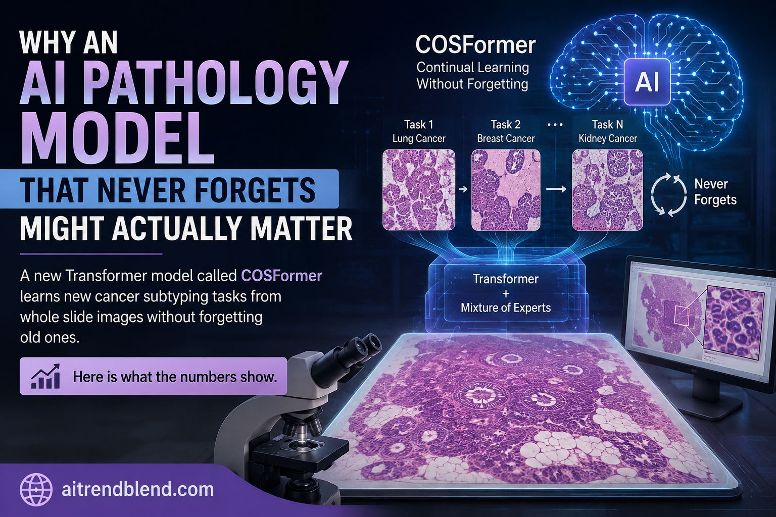
- Researchers from Korea University built COSFormer, a Transformer based model that learns new whole slide image tasks one at a time without retraining on prior datasets, tested across seven pathology datasets spanning six organs.
- When the model knows which task it is looking at, it reaches 93.137 percent average accuracy. When it does not know, that drops to 81.090 percent, a 12.047 percentage point gap that captures the real difficulty of this problem.
- A single design choice, replacing bare class labels like class0 and class1 with real diagnostic language like adenocarcinoma, improved accuracy by more than 70 percentage points on one dataset and rescued a task that otherwise scored a flat 0.000 percent.
- Every rival continual learning method tested lost far more accuracy when task identity was hidden. GDumb dropped nearly 40 percentage points, while COSFormer’s own drop stayed around 12 percentage points.
- The model still struggled on individual tasks at times, most visibly on TCGA-BRCA, where accuracy fell to 55.347 percent in one setting despite strong averages elsewhere.
- The full training and evaluation code is public, and every dataset used comes from open sources including the TCGA and CAMELYON16 archives.
Please read before continuing
This article explains a published computer science study on artificial intelligence and digitized pathology images. It is not medical advice, it is not a diagnosis, and it is not a treatment recommendation. Nothing here should be used to make decisions about an individual patient’s care. If you or someone you know has questions about a cancer diagnosis or pathology results, please talk with a qualified oncologist, pathologist, or other treating physician.
The problem hiding inside every pathology AI pilot program
Whole slide imaging turns a physical glass slide of tissue into a digital file that can be gigapixels in size, often more than ten thousand times larger than a typical photo used to train an everyday computer vision model. That scale alone forces pathology specific engineering. But size is not the only obstacle the researchers behind this paper, Doanh C. Bui and Jin Tae Kwak, point to. Pathology tasks are wildly varied. One task might detect whether cancer is present at all. Another grades how aggressive it looks. A third sorts tumors into molecular subtypes that guide treatment choice. And even though these tasks all draw on shared knowledge about how tissue looks under a microscope, most existing systems treat each one as a fresh, independent classification problem, throwing away any chance for one task to reinforce another.
Then there is the deployment reality that makes this paper worth reading closely. Hospitals are not going to hand over a fixed list of tasks once and be done. New diagnostic categories emerge, new organ systems get added to a pathology lab’s AI toolkit, and new patient cohorts arrive. Continual learning research exists to handle exactly this kind of ongoing change, letting a model absorb new tasks without needing the old training data ever again. The catch, well documented in the machine learning literature the authors cite, is catastrophic forgetting, where a model quietly loses its grip on what it learned previously the moment it is fine tuned on something new. Add in the fact that WSI datasets tend to be small relative to natural image datasets and you get a recipe for models that forget fast and generalize poorly.
What came before COSFormer
Two research threads converge in this paper. The first is multiple instance learning, or MIL, which is the standard way to squeeze a gigapixel slide into something a neural network can actually process. A WSI gets chopped into thousands of small patches, each patch becomes an embedding, and the model aggregates those embeddings into one prediction. ABMIL introduced simple attention weighting to highlight the patches that mattered most. CLAM refined that by also tracking the least useful patches. TransMIL brought Vision Transformer style long range attention into the mix so patches far apart on a slide could still inform each other. DTFD-MIL added a staged sub MIL branch specifically to help when sample sizes were small, and a more recent method called FALFormer improved how landmark patches get selected inside the attention mechanism. None of these methods, though, were built with an eye toward learning several tasks in sequence.
The second thread is continual learning itself, mostly developed outside of pathology. EWC constrains the parameters a model considers important so they cannot drift too far from where they sat after earlier training. GDumb takes almost the opposite approach, retraining from a small balanced memory buffer every time. ER-ACE rebalances the loss between old and new experience during replay. A-GEM constrains gradients so a new task cannot push performance on old tasks backward. DER++ pairs replay with a distillation style loss that keeps current predictions close to what the model previously predicted on the same samples. A pathology specific method called ConSlide pioneered continual learning built directly for WSIs using a strategy that breaks slides apart and reorganizes them to diversify what gets stored in a replay buffer. Other recent WSI focused approaches modeled the feature gap between current and buffered samples, or adapted vision language foundation models using a prototype pool matched against text descriptions of tumor classes.
All of these WSI tailored methods share a structural limitation the authors call out directly. They typically fix the number of class labels per task from the start, often just two cancer subtype classes, which works fine until a lab wants to add a task with three categories, or five, or one that overlaps partially with an earlier task’s vocabulary. That rigidity is the specific gap COSFormer tries to close.
How COSFormer actually works
COSFormer treats classification less like filling in a fixed set of output slots and more like writing a short diagnostic phrase, one word at a time, the way a language model generates text. That single design decision ripples through the entire architecture, and it is worth walking through the three components the authors build around it. You can read the complete architectural description and the full derivations in the open access paper on ScienceDirect, and the authors have also released working code on GitHub for anyone who wants to run it themselves.
Expert consultation, modeled on how doctors actually consult each other
Rather than dumping every learned task into one shared weight space, which is exactly what tends to blur together and cause interference between tasks, COSFormer keeps a dedicated expert for each task it has seen plus one generalist that oversees everything. When a new WSI comes in, a small router network looks at the patch embeddings and decides how much weight each expert should get. During training and during task aware inference, those weights get sharpened toward the correct target task using a scaling factor and a shifting factor, both tuned by hand. The experts are then combined into a single projection that transforms the raw patch features into the model’s working space. The authors describe this explicitly as inspired by real clinical consultations, where a generalist physician might loop in a kidney specialist for a kidney case and a lung specialist for a lung case, blending opinions rather than relying on one voice alone.
Autoregressive decoding instead of a fixed classification head
Most classifiers end with a linear layer that outputs one score per possible class, a design that requires knowing every class in advance and resizing that layer whenever a new class shows up. COSFormer swaps that out for a Transformer decoder borrowed conceptually from language models. It generates the diagnostic label word by word, starting from a beginning of sequence token and stopping at an end of sequence token, pulling each next word from a vocabulary that simply grows as new tasks and new class descriptions arrive. Practically, this means the word invasive ductal carcinoma gets treated the same way whichever task it shows up in, and adding a brand new organ with brand new subtype names never requires touching the model’s core architecture.
A buffer that remembers by meaning, not by chance
Like most rehearsal based continual learning systems, COSFormer keeps a small buffer of past WSIs to replay while learning new tasks, capped here at 26 slides total. What differs is how those 26 slides get chosen. Instead of randomly swapping slides in and out, which is what most earlier rehearsal methods do, COSFormer uses a visual encoder called UNI and a text encoder called PubMedBERT to score how well each candidate slide’s patches match the text description of its class, such as adenocarcinoma. It then clusters slides within each class using k means and keeps the highest scoring slide from each cluster, which the authors argue produces a buffer that is both representative of the class and diverse across visual variation. During training on a new task, the model is optimized against three combined signals, correct classification on the new task’s own data, correct classification on the buffer’s older data, and a consistency loss that pulls current predictions toward what a past version of the model would have predicted on that same buffered data.
How the expert committee gets blended into one projection
$$\theta_{EC} = \theta_{general} + \sum_{i=1}^{N_T} \theta_i \cdot \bar{w}_i$$The generalist weights \(\theta_{general}\) get combined with every task specific expert \(\theta_i\), each scaled by a refined routing weight \(\bar{w}_i\) that the router computes per WSI. This combined projection then transforms raw patch embeddings into the space the Transformer encoder actually works in.
Generating the diagnosis one word at a time
$$\hat{p}^{(k+1)} = Dec\big(Enc(z’) \mid \hat{p}^{(k)}\big)$$The decoder predicts the next word of the diagnostic term using the encoded slide features and everything predicted so far, exactly the pattern used to generate text in a language model, just applied here to produce a pathology label.
The three part training signal behind past to present learning
$$ \underbrace{CE(p^{(k)}_{t,i}, y^{(k)}_i \mid x_i \in D_t)}_{\text{learn the new task}} + \underbrace{CE(p^{(k)}_{t,i}, y^{(k)}_i \mid x_i \in B_r) + MSE(p^{(k)}_{t,i}, p^{(k)}_{<t,i} \mid x_i \in B_r)}_{\text{replay old tasks, and stay consistent with the past}} $$Cross entropy on the current task, cross entropy on buffered examples from earlier tasks, and a mean squared error term that discourages the model’s predictions on old data from drifting too far from what it used to predict. All three terms fire together during every training step on a new task.
How rigorously was this actually tested
The benchmark the authors assembled covers seven WSI datasets across six organs and seven distinct tasks. CAMELYON16 provides 160 tumor and 239 non tumor slides for breast lymph node metastasis detection. From The Cancer Genome Atlas, TCGA-NSCLC offers 109 adenocarcinoma and 845 squamous cell carcinoma lung slides. TCGA-BRCA covers 726 invasive ductal and 149 invasive lobular breast carcinoma slides. TCGA-RCC spans three kidney cancer subtypes, 289 papillary, 498 clear cell, and 118 chromophobe cases. TCGA-ESCA has 73 adenocarcinoma and 94 squamous cell carcinoma esophageal slides. TCGA-TGCT includes 150 seminoma and 55 mixed germ cell testicular tumor slides. TCGA-CESC rounds things out with 48 adenocarcinoma and 254 squamous cell carcinoma cervical and uterine slides.
Every experiment ran three times across different train, validation, and test splits to check for stability, and the model was trained on the tasks in a fixed sequence, first CAMELYON16 through TCGA-CESC and then reversed. Two evaluation conditions were used throughout. Under task aware evaluation, called TASK-IL in the paper, the model is told which task it is looking at and only has to choose among that task’s own classes. Under task blind evaluation, called CLASS-IL, the model gets no such hint and must pick the right answer out of every class it has ever learned across all tasks, which is a dramatically harder and arguably more realistic simulation of a real diagnostic workflow where the system does not always know in advance what kind of tissue it has been handed.
| Method | Task aware average | Task blind average | Accuracy lost going task blind |
|---|---|---|---|
| COSFormer | 93.137% | 81.090% | 12.047 points |
| DER++ | 92.180% | 71.198% | 20.982 points |
| ER-ACE | 82.997% | 69.627% | 13.370 points |
| LWSR | 84.285% | 66.551% | 17.734 points |
| A-GEM | 88.940% | 56.453% | 32.487 points |
| GDumb | 43.860% | 4.120% | 39.740 points |
Results shown for the CAMELYON16 to TCGA-CESC task sequence, drawn directly from the paper’s Table 1.
That table tells you most of what you need to know about why this paper matters more than a typical incremental accuracy bump. Every single rival method loses substantially more ground when task identity disappears. GDumb essentially collapses, dropping from a mediocre 43.860 percent down to a nearly useless 4.120 percent. COSFormer, by comparison, holds onto the large majority of its task aware performance even without being told what it is looking at, which is the scenario that most resembles an actual clinical pipeline receiving an unlabeled slide.
The word choice experiment that changed everything
One of the more revealing ablations in the paper tested what happens if you strip out the meaningful diagnostic language and replace it with arbitrary placeholders, so adenocarcinoma becomes class0 and squamous cell carcinoma becomes class1. Under task aware evaluation the difference was modest, sometimes even slightly favoring the naive labels on a couple of datasets. Under task blind evaluation the gap became enormous. On TCGA-ESCA, naive labels scored a flat 0.000 percent while semantic labels scored 90.996 percent. On TCGA-TGCT, semantic labels improved accuracy by 71.953 percentage points. On TCGA-NSCLC, the improvement was 65.943 percentage points. The authors’ explanation is that meaningful class descriptions let the autoregressive decoder share linguistic and conceptual structure across tasks, so that learning what adenocarcinoma looks like in lung tissue actually helps the model recognize adenocarcinoma in esophageal tissue later, since it is drawing on the same word and, presumably, some of the same underlying visual cues.
Worth remembering
The word choice ablation is arguably the single most practical finding in this paper for anyone building similar systems. It suggests that treating diagnostic categories as meaningful medical language rather than arbitrary integers is not a stylistic nicety, it measurably determines whether a model can generalize once task identity is unknown, which is the exact condition under which most real deployment failures would happen.
Where COSFormer’s advantage gets shaky
The paper is refreshingly candid about where the model struggles, and this is worth sitting with rather than skipping past. On TCGA-BRCA, COSFormer’s per task accuracy fell to 55.347 percent in the forward sequence and 47.942 percent in the reverse sequence under task blind evaluation, despite the model’s strong overall averages. Routing analysis later in the paper offers a partial explanation. When the authors measured how often the router correctly identified which expert should dominate for a given slide, success rates ranged from a perfect 100 percent on CAMELYON16 down to 60.0 percent on TCGA-TGCT in one sequence, and the router failed outright to correctly identify TCGA-ESCA and TCGA-CESC as distinct tasks, instead confusing them with TCGA-NSCLC. The reason traces back to shared vocabulary. TCGA-NSCLC, TCGA-ESCA, and TCGA-CESC all use the same two class names, adenocarcinoma and squamous cell carcinoma, despite covering completely different organs, lung, esophagus, and the uterine cervix respectively. That overlap helps performance in some cases, since knowledge genuinely transfers between related tasks, but it actively confuses the router in others, and the paper does not fully resolve which effect wins on which dataset.
What this looks like against models trained the old fashioned way
A fair question for any continual learning paper is whether all this complexity beats simply training a separate model per task, which sidesteps forgetting entirely at the cost of never sharing knowledge across tasks and requiring separate storage and maintenance for every model. The authors compared COSFormer against CLAM and TransMIL trained individually on each dataset. Under task aware evaluation on the forward sequence, individually trained CLAM-SB reached an average of 92.638 percent and TransMIL reached 93.253 percent, both very close to COSFormer’s 93.137 percent, with COSFormer actually surpassing both individually trained models on the CAMELYON16 and TCGA-CESC tasks specifically. Under task blind evaluation, though, the comparison flipped, with COSFormer generally trailing both individually trained MIL models, though it still beat them on TCGA-ESCA and TCGA-CESC. This is a genuinely fair result to report rather than cherry pick around, and it tells a nuanced story. Continual learning earns its keep primarily in the task blind scenario and in the practical benefits of maintaining one adaptable model instead of an ever growing pile of separate ones, not necessarily by beating dedicated single task models on their own turf every single time.
As the label space expands, logit diversity increases, which may introduce prediction ambiguity when explicit task identity is unavailable. Paraphrased from the paper’s discussion of why the class blind scenario proved harder for the model’s individual components, Bui and Kwak, Medical Image Analysis, 2026
The clinical translation gap
Everything described above happened inside a research pipeline running on TCGA and CAMELYON16 data, curated collections assembled specifically for algorithm development, evaluated on an NVIDIA A6000 GPU under controlled experimental conditions. Getting from that setting to a functioning tool inside an actual pathology department involves several gaps this paper does not close, and it would be misleading to imply otherwise.
First, TCGA slides come from multiple institutions but were collected as a research resource, and prior work the authors themselves cite has shown that site specific scanner and staining differences can meaningfully shift how a model performs, sometimes described as digital histology signatures distinct from the actual biology. A model validated on TCGA is not automatically validated for a specific hospital’s scanner, staining protocol, or patient population. Second, this study evaluates cancer subtyping and metastasis detection, both classification tasks. Many of the clinical questions pathologists actually answer, like predicting treatment response, recurrence risk, or survival, involve different task structures the authors explicitly flag as future work rather than something this paper addresses. Third, nothing in this study involved prospective clinical use, regulatory review, or comparison against a working pathologist’s diagnostic accuracy on the same slides in a live setting. The reported accuracies describe how well the model matches existing ground truth labels in a research benchmark, which is a meaningfully different question from how the model would perform, or should be trusted, inside an actual diagnostic workflow making decisions that affect real patients.
Honest limitations, in the authors’ own words and numbers
The paper includes an unusually long and specific limitations discussion, and it is worth walking through rather than summarizing away. COSFormer did not win on every individual task, with TCGA-BRCA standing out as a case where task blind accuracy dropped well below the model’s overall average. The benchmark covers seven datasets and six organs, a meaningful scope but still narrow relative to the full range of cancer types and non cancer pathology tasks that exist. Only two task orderings were tested, forward and reverse, leaving open how the model would behave under more varied or randomized sequences. As new tasks accumulate, the model’s parameter count grows too, since each new task adds its own expert matrix and new vocabulary words, and while the authors describe this growth as small relative to overall model size, they acknowledge it could become a scalability concern across many more tasks than the seven tested here. The autoregressive decoding step, generating labels word by word rather than in one pass, adds inference latency compared to a standard linear classifier, though the authors note this cost is modest next to the computational load of extracting and aggregating features from a gigapixel slide in the first place.
Two limitations stand out as particularly relevant to anyone thinking about real deployment. The model performs consistently better when it knows the target task than when it does not, and the routing mechanism that tries to infer task identity on its own is not fully reliable, especially among tasks that happen to share diagnostic vocabulary. And nearly all the data used comes from TCGA, which despite spanning multiple contributing institutions is still a research archive rather than a live, continuously updating multi institutional clinical data stream with the scanner diversity, staining variation, and patient population breadth a production deployment would actually encounter. The authors explicitly name extending evaluation to non TCGA, multi institutional clinical cohorts as necessary future work, not something this study has already established.
Reference implementation of the core architecture
What follows is a compact PyTorch implementation that mirrors the architecture described in the paper, the expert consultation routing mechanism, a Transformer encoder over patch embeddings, and an autoregressive Transformer decoder that produces diagnostic words one step at a time, trained with the three part past to present loss. It is written for learning and experimentation on your own data, not as a drop in clinical tool, and it does not include the visual and text encoders, UNI and PubMedBERT, that the original authors use for feature extraction and buffer retrieval, since those are large pretrained models loaded separately in the official release linked above.
# Reference implementation of the COSFormer architecture described in this article
# Educational scaffold, not the authors original codebase, see the GitHub link for that

import torch
import torch.nn as nn
import torch.nn.functional as F
import math

class ExpertConsultation(nn.Module):
    """Routes a bag of patch embeddings through a generalist plus a growing committee of task experts."""
    def __init__(self, feat_dim, model_dim, gamma=5.0, beta=1.0):
        super().__init__()
        self.feat_dim = feat_dim
        self.model_dim = model_dim
        self.gamma = gamma
        self.beta = beta
        self.generalist = nn.Parameter(torch.randn(feat_dim, model_dim) * 0.02)
        self.experts = nn.ParameterList()
        self.router_fc1 = None
        self.router_fc2 = None

    def add_task(self, num_tasks_so_far):
        """Called once whenever a brand new task arrives, following Algorithm 1 in the paper."""
        new_expert = nn.Parameter(torch.randn(self.feat_dim, self.model_dim) * 0.02)
        self.experts.append(new_expert)
        hidden = max(self.feat_dim // 2, 16)
        self.router_fc1 = nn.Linear(self.feat_dim, hidden)
        self.router_fc2 = nn.Linear(hidden, num_tasks_so_far)

    def forward(self, z, target_task_idx=None, task_aware=True):
        # z has shape num_patches by feat_dim for a single slide
        num_tasks = len(self.experts)
        raw_weights = self.router_fc2(F.relu(self.router_fc1(z)))
        if task_aware and target_task_idx is not None:
            mask = torch.zeros_like(raw_weights)
            mask[:, target_task_idx] = self.gamma
            scaled = raw_weights + mask
        else:
            scaled = raw_weights
        w_soft = F.softmax(scaled, dim=1)
        w_bar = w_soft.mean(dim=0)
        if task_aware and target_task_idx is not None:
            w_bar = w_bar.clone()
            w_bar[target_task_idx] = w_bar[target_task_idx] + self.beta
        theta_ec = self.generalist.clone()
        for i, expert in enumerate(self.experts):
            theta_ec = theta_ec + expert * w_bar[i]
        return z @ theta_ec, w_bar


class SlideEncoder(nn.Module):
    """A standard Transformer encoder stack over patch embeddings, standing in for the Nystrom attention used in the paper."""
    def __init__(self, model_dim, num_layers=2, num_heads=8):
        super().__init__()
        layer = nn.TransformerEncoderLayer(d_model=model_dim, nhead=num_heads, batch_first=True)
        self.encoder = nn.TransformerEncoder(layer, num_layers=num_layers)

    def forward(self, z):
        return self.encoder(z)


class AutoregressiveDecoder(nn.Module):
    """Generates a diagnostic term one word at a time, cross attending to the encoded slide patches."""
    def __init__(self, model_dim, vocab_size, num_layers=2, num_heads=8, max_len=8):
        super().__init__()
        self.word_embed = nn.Embedding(vocab_size, model_dim)
        self.pos_embed = nn.Embedding(max_len, model_dim)
        layer = nn.TransformerDecoderLayer(d_model=model_dim, nhead=num_heads, batch_first=True)
        self.decoder = nn.TransformerDecoder(layer, num_layers=num_layers)
        self.out_proj = nn.Linear(model_dim, vocab_size)

    def forward(self, encoded_patches, prev_word_ids):
        seq_len = prev_word_ids.shape[1]
        positions = torch.arange(seq_len, device=prev_word_ids.device).unsqueeze(0)
        h = self.word_embed(prev_word_ids) + self.pos_embed(positions)
        causal_mask = nn.Transformer.generate_square_subsequent_mask(seq_len).to(h.device)
        h = self.decoder(tgt=h, memory=encoded_patches, tgt_mask=causal_mask)
        return self.out_proj(h)


class COSFormerLite(nn.Module):
    """Wires the three components together, following Eqs. 1 through 7 and Algorithm 1 in the paper."""
    def __init__(self, feat_dim=1024, model_dim=512, vocab_size=64, max_len=8):
        super().__init__()
        self.ec = ExpertConsultation(feat_dim, model_dim)
        self.enc = SlideEncoder(model_dim)
        self.dec = AutoregressiveDecoder(model_dim, vocab_size, max_len=max_len)

    def forward(self, patch_embeddings, prev_word_ids, target_task_idx=None, task_aware=True):
        z_proj, w_bar = self.ec(patch_embeddings, target_task_idx=target_task_idx, task_aware=task_aware)
        z_proj = z_proj.unsqueeze(0)
        encoded = self.enc(z_proj)
        logits = self.dec(encoded, prev_word_ids)
        return logits, w_bar


def past_to_present_loss(logits_current, targets_current, logits_buffer=None, targets_buffer=None, logits_buffer_past=None):
    """Implements Eq. 14, the three term loss behind past to present learning."""
    loss = F.cross_entropy(logits_current.reshape(-1, logits_current.shape[-1]), targets_current.reshape(-1))
    if logits_buffer is not None:
        loss = loss + F.cross_entropy(logits_buffer.reshape(-1, logits_buffer.shape[-1]), targets_buffer.reshape(-1))
    if logits_buffer_past is not None:
        loss = loss + F.mse_loss(logits_buffer, logits_buffer_past)
    return loss


def smoke_test():
    torch.manual_seed(0)
    model = COSFormerLite(feat_dim=1024, model_dim=512, vocab_size=20, max_len=5)
    model.ec.add_task(num_tasks_so_far=1)
    num_patches = 100
    patch_embeddings = torch.randn(num_patches, 1024)
    prev_word_ids = torch.randint(0, 20, (1, 4))
    logits, w_bar = model(patch_embeddings, prev_word_ids, target_task_idx=0, task_aware=True)
    targets = torch.randint(0, 20, (1, 4))
    loss = past_to_present_loss(logits, targets)
    loss.backward()
    print(f"Smoke test complete. Logit shape {tuple(logits.shape)}. Loss value {loss.item():.4f}. Router weights {w_bar.detach().numpy()}")


if __name__ == "__main__":
    smoke_test()
Conclusion
Strip away the equations and what COSFormer really argues is that continual learning in pathology should stop pretending every task is a clean, fixed, isolated classification problem. Cancer diagnosis language is shared across organs in ways a rigid class list cannot capture, adenocarcinoma means something related whether it shows up in lung tissue or esophageal tissue, and a model that can lean on that shared vocabulary through autoregressive decoding picks up real transfer benefits that a model locked into per task output heads simply cannot access. The expert consultation mechanism, meanwhile, tackles the opposite risk, making sure that shared vocabulary and shared architecture do not collapse every task’s specific visual signature into one blurry average representation.
The conceptual shift worth sitting with is the move from classification as a fixed lookup table to classification as language generation. That reframing is what lets the vocabulary grow gracefully as new tasks and new class names arrive, without touching the core network architecture or resizing an output layer every time a lab wants to add a new cancer type. It is a genuinely different way to think about what a diagnostic classifier even is, treating a diagnosis less like picking one of N boxes and more like producing an accurate, structured piece of medical language.
On transferability, very little about the expert consultation and autoregressive decoding combination is specific to pathology. Any domain with a stream of related classification tasks that share meaningful label vocabulary, radiology subtyping, dermatology lesion classification, or even non medical multi task image classification problems, could plausibly borrow this architecture. The text based buffer retrieval strategy in particular, choosing what to remember based on vision language similarity rather than random sampling, seems like a broadly useful idea for continual learning generally, not just for slides.
The honest remaining limitations matter more here than in most computer science papers, precisely because the application touches cancer diagnosis. Task blind performance, the setting that most resembles a real unlabeled clinical input, still trails task aware performance by a meaningful margin, the routing mechanism that is supposed to infer task identity on its own fails on datasets with overlapping vocabulary, individual task performance varies more than the strong averages suggest, and every dataset used comes from research archives rather than a live multi institutional clinical pipeline. None of that erases what the paper accomplishes. It does mean the responsible reading of this work is as a meaningful step in continual learning research for pathology, not as a validated clinical tool.
Where this goes next, based on the authors’ own stated direction, likely involves broadening beyond flat cancer subtype classification into hierarchical diagnostic structures, extending into detection and segmentation tasks rather than just classification, and testing on genuinely diverse, non TCGA clinical cohorts with the scanner and staining variability that real hospitals actually produce. Until that broader validation exists, the fair way to describe COSFormer is as a well tested, honestly reported research architecture that points toward a more flexible way of building pathology AI systems, not as evidence that any such system is ready for a diagnostic workflow today.
If you take one thing from this
The gap between 93.137 percent task aware accuracy and 81.090 percent task blind accuracy is the number that matters most if you are evaluating any continual learning claim in medical imaging. Ask whether a reported accuracy assumes the model already knows what it is looking at, because that assumption rarely holds in a real clinical pipeline receiving an unlabeled sample.
Frequently asked questions
What is COSFormer and what problem does it solve
COSFormer is a Transformer based continual learning model for whole slide pathology image analysis, built by researchers at Korea University. It lets a single model learn new cancer subtyping tasks over time without retraining on previously seen datasets, addressing the common problem of catastrophic forgetting in machine learning.
How accurate is COSFormer compared to other continual learning methods
Across seven whole slide image datasets, COSFormer reached average accuracies of 93.137 percent and 91.140 percent under task aware evaluation for two different task orderings, and 81.090 percent and 79.359 percent under the harder task blind evaluation, outperforming five comparison methods including GDumb, ER-ACE, A-GEM, DER++, and LWSR in every setting tested.
Is COSFormer ready to be used for real cancer diagnosis
No. This is a research study evaluated on publicly available research datasets including TCGA and CAMELYON16, under experimental conditions, without prospective clinical testing or regulatory review. The authors themselves identify multi institutional clinical validation as necessary future work. It should not be used or interpreted as a diagnostic tool.
Why did using real medical words instead of arbitrary labels matter so much
When the researchers replaced diagnostic terms like adenocarcinoma with arbitrary placeholders like class0, accuracy collapsed under task blind evaluation, including a complete failure on one dataset. Meaningful medical language appears to let the model transfer shared knowledge across tasks that use the same diagnostic terms, which arbitrary labels cannot provide.
What datasets and organs does this research cover
The benchmark spans seven datasets and six organs, CAMELYON16 for breast lymph node metastasis, and TCGA cohorts for lung, breast, kidney, esophageal, testicular, and cervical or uterine cancer subtyping, totaling several thousand whole slide images across all seven datasets combined.
Where can I read the full study or see the code
The complete paper is published in Medical Image Analysis and is openly accessible through its DOI. The authors have also released their training and evaluation code publicly on GitHub, linked in the call to action section of this article.
Read the full methodology, every table, and the complete reference list.
Read the full paper View the official code on GitHubSource. Bui, D.C. and Kwak, J.T. Welcome new doctor, continual learning with expert consultation and autoregressive inference for whole slide image analysis. Medical Image Analysis, Volume 114, 2026, Article 104235. Published under CC BY NC ND 4.0. DOI 10.1016/j.media.2026.104235. Code available at github.com/QuIIL/COSFormer.
This analysis is based on the published paper and an independent evaluation of its claims.