
Key points
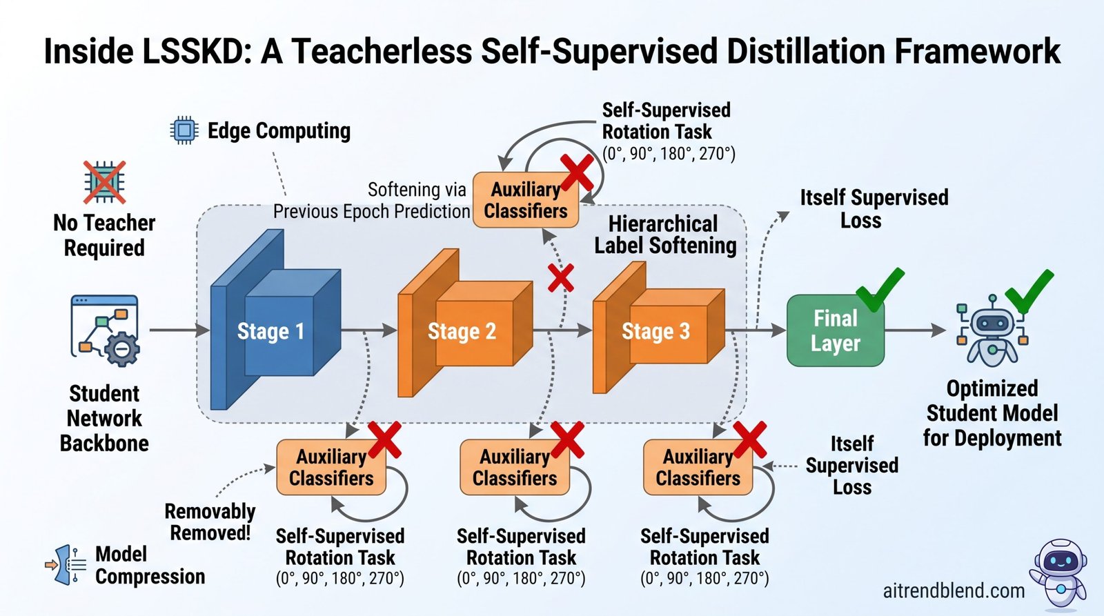
- LSSKD, short for Layered Self Supervised Knowledge Distillation, trains a compact model with no teacher network at all, instead attaching temporary auxiliary classifiers to each stage of the student itself.
- Those auxiliary classifiers learn a self supervised task built from image rotations, and their predictions from the previous training epoch are used to soften the hard labels for the current epoch, at every stage of the network, not just the last one.
- On CIFAR 100 with a ResNet34 to ResNet18 pair, LSSKD reaches 72.45 percent top 1 accuracy against a 69.75 percent baseline, edging out every listed prior method in the paper’s main comparison table.
- All auxiliary branches are deleted after training, so the deployed model costs exactly the same to run as an ordinary ResNet18, with none of the training time scaffolding left behind.
- The paper’s own numbers are not perfectly consistent between the abstract, the results section and one of the result tables, which is worth knowing before quoting any single headline percentage from it.
The pitch, distillation without a teacher to babysit
Knowledge distillation has a well known shape. Train a large, accurate teacher model. Train a small student model to mimic the teacher’s softened output probabilities, using the temperature trick Geoffrey Hinton popularized, rather than only the ground truth labels. The student ends up more accurate than it would be from label supervision alone, because the teacher’s probability distribution over wrong answers carries information a one hot label cannot, sometimes called dark knowledge.
The catch is that a teacher model is itself an expensive thing to own. It has to be trained, stored and kept around during every student training run, and on genuinely resource constrained hardware, even that offline cost can be a real barrier. A line of research called self distillation sidesteps the problem entirely by having a model learn from its own past predictions instead of a separate teacher. Progressive Self Knowledge Distillation, referred to throughout the paper as PS-KD, is one of the better known examples, using a model’s own predictions from a previous epoch as a softening signal for the current epoch’s targets.
A team spanning Pakistan’s National University of Computer and Emerging Sciences, Universiti Malaya, Hong Kong Polytechnic University, COMSATS University, the University of Tennessee Oak Ridge Innovation Institute, and the University of Central Florida, argues that PS-KD and similar methods are leaving something on the table. They only ever soften the final layer’s predictions. Every intermediate stage of a convolutional network, the layers that build up the visual hierarchy from edges to textures to object parts, gets skipped entirely. LSSKD is their attempt to bring that same progressive softening down into the middle of the network, not just its output.
If softened labels genuinely help a network generalize, and the evidence from PS-KD and earlier work suggests they do, then applying that softening only at the final classifier is arguably wasting the technique on one layer out of many. LSSKD is a test of whether spreading the same idea across every stage compounds the benefit or just adds training overhead for a marginal gain.
How the architecture is put together
The backbone of LSSKD is an ordinary convolutional network, described in the paper using the standard split of a feature extractor and a final linear classifier. What makes it different is what gets bolted on during training and stripped off before deployment.
Auxiliary branches at every stage
After each of the network’s bottleneck stages, typically three stages for the architectures tested here, LSSKD attaches a small auxiliary branch, each one containing its own feature extraction module, a global average pooling layer, and a linear classifier. The authors note this design choice was deliberate. An earlier ablation from other researchers found that a bare linear classifier attached directly to raw intermediate features, without its own small feature extraction step first, fails to pull out anything meaningful. Giving each auxiliary branch a bit of its own processing capacity turned out to matter.
A self supervised task built from rotations
Rather than training these auxiliary branches on the same N way classification task as the main classifier, LSSKD gives them a harder, self generated task. Every training image is rotated by 0, 90, 180 and 270 degrees, producing four transformed versions. Each auxiliary classifier then has to predict both the original class and which of the four rotations was applied, jointly, which multiplies the label space from N classes to N times M classes, 400 combined labels for the 100 classes of CIFAR 100 with four rotations. This forces the intermediate layers to encode more than category identity, since telling a rotated bird from an upright bird requires the network to represent orientation, something a plain classification loss has no reason to preserve on its own.
Here q is the self supervised augmented distribution, or SAD in the paper’s shorthand, produced by a given auxiliary classifier at softmax temperature tau, over the full N times M joint label space.
Where the softening actually happens
The heart of the method is what the paper calls hierarchical label softening, and it works across two axes at once, network depth and training time. The mechanism is best understood as the student network mimicking its own predictions from one epoch earlier, at every stage simultaneously, illustrated in the paper as a comparison between the student backbone at epoch e and the same backbone frozen at epoch e minus 1.
Softening the final classifier’s targets
For the deepest, final classifier, the soft target for the current epoch blends the original one hot label with the model’s own prediction from the previous epoch.
This is close in spirit to what PS-KD already does. Alpha controls how much of the previous epoch’s own confidence gets folded into this epoch’s target, and the paper settles on alpha equal to 0.8 after tuning on a held out validation split, meaning the model leans fairly heavily on its own recent history rather than the raw one hot label.
Softening every auxiliary classifier’s targets too
The novel part is doing the same thing at every intermediate stage, using each stage’s own previous epoch prediction on the rotated, self supervised task.
The paper visualizes this blending step as a small module it names the hybrid self supervised fusion module, which takes the previous epoch’s distribution for a given stage, adjusts it against the true target, weights the result by alpha, and outputs the current epoch’s soft label for that stage. The practical effect is that every auxiliary classifier gets its own progressively refined target, not just a copy of whatever the final layer decided.
Passing knowledge from deep stages back to shallow ones
A separate mechanism moves information sideways within a single epoch rather than across epochs. A Kullback Leibler divergence term encourages each shallow auxiliary classifier’s self supervised distribution to move toward the deepest classifier’s self supervised distribution, on the theory that deeper layers have already learned a more useful representation and earlier layers should be nudged to agree with them.
Alongside this, a second term pulls the actual feature maps closer together rather than just the output probabilities, computing an L2 distance between each auxiliary stage’s pooled feature map and the final layer’s pooled feature map, encouraging what the paper calls internal consistency between the intermediate representations and the representation the network ultimately settles on.
Combining everything into one training objective
The paper groups its five loss terms into two families. A Label Supervised loss, combining the responsive cross entropy on the final classifier’s softened targets with the hierarchical cross entropy across all the auxiliary stages, and what it calls an Itself Supervised loss, combining the deep to shallow KL divergence with the feature consistency term. The two families are summed with two extra hyperparameters, beta and gamma, controlling how much weight the network gives to the self referential terms relative to the label based ones.
The final values used across every experiment were alpha at 0.8, beta at 0.1 and gamma at 0.1, tuned using a 10 percent held out validation split carved out of the training data. Notice how small beta and gamma are relative to the label based terms, which suggests the bulk of the benefit is coming from the softened label targets rather than the auxiliary regularization terms, a point the paper’s own ablation study later supports.
What the results actually show
The headline comparison sits in Table I of the paper, training a ResNet18 student under a ResNet34 teacher’s shadow, except there is no teacher actually involved in training LSSKD itself, the ResNet34 numbers are included only so readers can see the usual ceiling a teacher based method would be chasing.
| Method | Top 1 accuracy | Top 5 accuracy |
|---|---|---|
| Student baseline, ResNet18, no distillation | 69.75 | 89.07 |
| Original KD, Hinton style | 70.66 | 89.88 |
| SSKD, self supervised distillation with a teacher | 71.62 | 90.67 |
| HSSAKD, hierarchical augmented self supervised distillation | 72.16 | 90.85 |
| MOKD | 72.3 | 90.9 |
| LSSKD, the paper’s proposed method | 72.45 | 91.15 |
| Teacher, ResNet34, for reference only | 73.31 | 91.42 |
LSSKD edges out every baseline listed in that table on both metrics, and it does so while never once consulting a trained teacher network during the student’s training. A second, broader comparison in Table II runs six different teacher and student architecture pairs, from a WRN-40-2 down to a WRN-16-2, through ResNet56 down to ResNet20, up to the more unusual case of distilling a WRN-40-2 into a lightweight ShuffleNetV1. LSSKD comes out ahead of every other method the authors compare against in every one of those six pairings, though by varying margins, the largest gap opening up on the ResNet32x4 to ShuffleNetV2 pairing, where LSSKD reaches 79.43 percent against the next best result of 78.26 percent from a method called SemCKD.
All auxiliary branches can be removed at inference, yielding no extra computational cost. Paraphrased from the paper’s abstract and Section III.D conclusion
A closer look at the self distillation specific comparison
Table III narrows the field to methods that, like LSSKD, use no separate teacher at all, comparing against label smoothing, CSKD, the teacher free Tf-KD variant, and PS-KD, across ResNet18, ResNet101 and MobileNetV2 students. Here the reported gap widens considerably. LSSKD reaches 83.16 percent on ResNet18 against a 75.87 percent baseline and PS-KD’s 79.18 percent, and 73.95 percent on MobileNetV2 against a 68.38 percent baseline. Those are large jumps, five to eight points over the next best self distillation method depending on the architecture, and worth treating with a little more scrutiny than the smaller, more typical single point gains reported elsewhere in the paper.
It is also worth flagging something the paper itself does not address directly. Table III labels its own proposed method column MSAKD rather than LSSKD, and Table IV does the same. Every other table and the entire body of the paper uses the LSSKD name consistently. This reads like a naming artifact left over from an earlier version of the project rather than a second, undocumented method, but a careful reader should not assume the two names definitely refer to identical runs without the authors clarifying it.
The abstract’s numbers do not quite match the body text
A second inconsistency worth naming plainly. The abstract states LSSKD achieves an average improvement of 4.54 percent over PS-KD and a 1.14 percent gain over SSKD on CIFAR 100. The results section, in its overall performance discussion, instead states LSSKD achieves an average improvement of 4.54 percent over SSKD, attributing the same 4.54 figure to a different baseline than the abstract does. The paper’s own contributions list in the introduction states yet a third framing, 4.54 percent over PS-KD and 1.14 percent over SSKD, which at least matches the abstract. On ImageNet, the abstract reports a 0.32 percent gain over HASSKD, while the results section reports a 0.33 percent top 1 gain without naming a comparison method in that particular sentence. None of this changes the overall conclusion that LSSKD compares favorably against the listed baselines, the accuracy tables back that up on their own, but a reader quoting a specific headline percentage from this paper should pull it from Table I or Table II directly rather than from the prose, since the prose is not fully self consistent.
Testing generalization when labeled data is scarce
Beyond the standard full data benchmarks, the authors ran a few shot style test, keeping 25, 50 and 75 percent of the CIFAR 100 and Tiny ImageNet training sets while leaving the test sets untouched, using stratified sampling so every class stays represented at each data fraction. On Tiny ImageNet, using a ResNet56 teacher shaped architecture distilled into a ResNet20 shaped student, LSSKD topped every comparison method at every data fraction tested, reaching 50.1 percent accuracy at 25 percent of the training data, 53.5 percent at 50 percent, and 54.5 percent at 75 percent, ahead of KD, CRD, SSKD and HSSAKD at each point on that curve. The gap over the plain KD baseline is largest in the most data scarce setting, at 25 percent of the training data, which is a reasonable argument that the self supervised auxiliary task is doing something more than just squeezing a bit more accuracy out of abundant labels, it appears to be providing a useful supervisory signal precisely when labeled examples are hardest to come by.
Reading the ablation study honestly
The paper’s ablation section is thinner than its main results section, but it does make two specific, checkable claims. First, a stagewise comparison against a closely related prior method called HASKD, shown as a bar chart contrasting accuracy at each auxiliary stage. Across both a ResNet32x4 based setup and a ResNet18 based setup, LSSKD’s auxiliary classifiers score noticeably higher at every intermediate stage than HASKD’s do, roughly in the 80 to 81 percent range for LSSKD’s early stage classifiers against the low to mid 70s for HASKD’s equivalent stages in the paper’s own chart. That is a meaningfully large gap for what is ostensibly a comparison of two closely related label softening designs, and the paper attributes it to the deepest classifier being a stronger supervisory source than the fixed hard labels HASKD relies on.
Second, Table IV reports the accuracy gain LSSKD adds over an untouched baseline architecture across six backbones, without a distillation baseline like PS-KD or SSKD in the same table for direct comparison, which makes the table read more like an internal consistency check than a competitive benchmark.
| Backbone | Baseline accuracy | LSSKD accuracy | Gain |
|---|---|---|---|
| ResNet20 | 69.62 | 72.67 | +3.05 |
| ResNet56 | 71.83 | 78.79 | +3.96 |
| WRN-16-2 | 76.77 | 83.16 | +6.39 |
| WRN-40-2 | 76.89 | 85.68 | +8.79 |
| ResNet18 | 73.57 | 76.89 | +3.32 |
| ResNet50 | 75.81 | 82.63 | +6.22 |
The pattern across this table is fairly consistent, wider networks such as the WRN family gain more from the layered self supervision than the plain ResNet family does, which fits a reasonable intuition that a network with more channels per stage has more room for an auxiliary classifier to extract a genuinely separate signal from, rather than fighting the main classifier for the same limited feature capacity.
What the paper is honest about not knowing yet
To its credit, the limitations section is short but specific rather than a vague gesture at future work. The authors flag three open questions directly. Whether the method holds up on datasets meaningfully larger than CIFAR 100, Tiny ImageNet and the single ResNet18 ImageNet run reported here remains untested. Whether the approach transfers past image classification into object detection, machine translation or other model compression settings is left entirely for future work, meaning every claim in this paper about generalization is currently scoped to classification alone. And the authors note that the auxiliary branches themselves, while removed at inference, still add meaningful training time and memory overhead during the training run itself, an angle they suggest could be addressed by pruning some of the deeper auxiliary structure without giving up the accuracy gain.
The core trade this paper is making is training time complexity in exchange for zero inference time complexity. Every auxiliary classifier, every rotation augmented forward pass, every epoch to epoch prediction cache adds cost while the model is being trained, and none of it survives into the deployed model. For edge deployment specifically, where inference cost is what actually matters on the device, that is close to the ideal shape for a training trick to take.
Full PyTorch style implementation
The block below sketches the core mechanics of LSSKD, an auxiliary branch module attached after each backbone stage, the rotation based self supervised augmentation, the hybrid self supervised fusion step that blends a target with the model’s own previous epoch prediction, the five loss terms combined into the total objective, a minimal training loop that caches predictions across epochs the way the method requires, and a runnable smoke test on random dummy tensors so the shapes can be checked without a real dataset. It is meant as a starting point for a reimplementation rather than a byte for byte reproduction of the authors’ original code.
# lsskd.py
# Educational reimplementation of the LSSKD framework
# Dahri et al., arXiv 2506.07055, 2025
# Not affiliated with the original authors, defaults chosen for clarity

import torch
import torch.nn as nn
import torch.nn.functional as F


# ---------------------------------------------------------------
# Auxiliary branch attached after a backbone stage, contains its
# own small feature extractor rather than a bare linear layer,
# matching the paper's note in Section III.A
# ---------------------------------------------------------------
class AuxiliaryBranch(nn.Module):
    def __init__(self, in_channels, num_classes, num_transforms=4, hidden_channels=128):
        super().__init__()
        self.feature_extractor = nn.Sequential(
            nn.Conv2d(in_channels, hidden_channels, kernel_size=3, padding=1),
            nn.BatchNorm2d(hidden_channels),
            nn.ReLU(inplace=True),
        )
        self.pool = nn.AdaptiveAvgPool2d(1)
        # output dimension is N times M, the joint class and transform label space
        self.classifier = nn.Linear(hidden_channels, num_classes * num_transforms)
        self.num_classes = num_classes
        self.num_transforms = num_transforms

    def forward(self, feature_map):
        h = self.feature_extractor(feature_map)
        pooled = self.pool(h).flatten(1)
        logits = self.classifier(pooled)
        return logits, pooled


# ---------------------------------------------------------------
# Applies the four rotation transforms used as the self supervised
# pretext task, 0, 90, 180 and 270 degrees, Section III.A
# ---------------------------------------------------------------
def make_rotated_batch(images):
    # images shape, batch, channels, height, width
    rotations = [images]
    for k in (1, 2, 3):
        rotations.append(torch.rot90(images, k=k, dims=[2, 3]))
    # stacked shape, batch times 4, channels, height, width
    return torch.cat(rotations, dim=0)


# ---------------------------------------------------------------
# Hybrid self supervised fusion module, Figure 4 in the paper,
# blends the previous epoch's distribution with the true target
# weighted by alpha to produce the current epoch's soft label
# ---------------------------------------------------------------
def hybrid_soft_label(previous_epoch_dist, one_hot_target, alpha=0.8):
    return (1.0 - alpha) * one_hot_target + alpha * previous_epoch_dist


# ---------------------------------------------------------------
# The five loss terms from Equations 4, 5, 7 and 8, combined
# into the total objective from the final equation in Section III.D
# ---------------------------------------------------------------
def responsive_ce_loss(final_logits, soft_target):
    log_probs = F.log_softmax(final_logits, dim=-1)
    return -(soft_target * log_probs).sum(dim=-1).mean()


def hierarchical_ce_loss(aux_logits_list, soft_target_list):
    total = 0.0
    for logits, target in zip(aux_logits_list, soft_target_list):
        log_probs = F.log_softmax(logits, dim=-1)
        total = total + (-(target * log_probs).sum(dim=-1).mean())
    return total / len(aux_logits_list)


def deep_to_shallow_kl_loss(aux_logits_list, deepest_logits, temperature=4.0):
    deepest_probs = F.softmax(deepest_logits / temperature, dim=-1).detach()
    total = 0.0
    for logits in aux_logits_list:
        log_probs = F.log_softmax(logits / temperature, dim=-1)
        kl = F.kl_div(log_probs, deepest_probs, reduction="batchmean")
        total = total + (temperature ** 2) * kl
    return total / len(aux_logits_list)


def feature_consistency_loss(aux_feature_list, final_feature):
    total = 0.0
    for feat in aux_feature_list:
        total = total + F.mse_loss(feat, final_feature.detach())
    return total / len(aux_feature_list)


def lsskd_total_loss(final_logits, soft_final_target, aux_logits_list, soft_aux_targets,
                     aux_feature_list, final_feature, beta=0.1, gamma=0.1):
    ce_resp = responsive_ce_loss(final_logits, soft_final_target)
    ce_heir = hierarchical_ce_loss(aux_logits_list, soft_aux_targets)
    div_sad = deep_to_shallow_kl_loss(aux_logits_list, final_logits)
    feat = feature_consistency_loss(aux_feature_list, final_feature)
    total = (1 - beta) * ce_resp + ce_heir + beta * div_sad + gamma * feat
    return total, {
        "ce_resp": ce_resp.item(), "ce_heir": ce_heir.item(),
        "div_sad": div_sad.item(), "feat": feat.item(),
    }


# ---------------------------------------------------------------
# A tiny three stage backbone, standing in for a real ResNet,
# with an auxiliary branch after each stage plus a final classifier
# ---------------------------------------------------------------
class LSSKDStudent(nn.Module):
    def __init__(self, num_classes=100, num_transforms=4, base_channels=32):
        super().__init__()
        self.stage1 = nn.Sequential(nn.Conv2d(3, base_channels, 3, padding=1), nn.BatchNorm2d(base_channels), nn.ReLU(inplace=True))
        self.stage2 = nn.Sequential(nn.Conv2d(base_channels, base_channels * 2, 3, stride=2, padding=1), nn.BatchNorm2d(base_channels * 2), nn.ReLU(inplace=True))
        self.stage3 = nn.Sequential(nn.Conv2d(base_channels * 2, base_channels * 4, 3, stride=2, padding=1), nn.BatchNorm2d(base_channels * 4), nn.ReLU(inplace=True))

        self.aux1 = AuxiliaryBranch(base_channels, num_classes, num_transforms)
        self.aux2 = AuxiliaryBranch(base_channels * 2, num_classes, num_transforms)
        self.aux3 = AuxiliaryBranch(base_channels * 4, num_classes, num_transforms)

        self.pool = nn.AdaptiveAvgPool2d(1)
        self.classifier = nn.Linear(base_channels * 4, num_classes)

    def forward(self, x):
        f1 = self.stage1(x)
        f2 = self.stage2(f1)
        f3 = self.stage3(f2)

        aux1_logits, aux1_feat = self.aux1(f1)
        aux2_logits, aux2_feat = self.aux2(f2)
        aux3_logits, aux3_feat = self.aux3(f3)

        pooled = self.pool(f3).flatten(1)
        final_logits = self.classifier(pooled)

        aux_logits_list = [aux1_logits, aux2_logits, aux3_logits]
        aux_feature_list = [aux1_feat, aux2_feat, aux3_feat]
        return final_logits, pooled, aux_logits_list, aux_feature_list


# ---------------------------------------------------------------
# A minimal training step that caches the previous epoch's
# predictions and blends them into this epoch's soft targets,
# following the progressive softening in Section III.B
# ---------------------------------------------------------------
def train_step(model, images, one_hot_labels, one_hot_aux_labels_list,
               previous_epoch_cache, optimizer, alpha=0.8, beta=0.1, gamma=0.1):
    model.train()
    optimizer.zero_grad()

    final_logits, final_feat, aux_logits_list, aux_feature_list = model(images)

    prev_final, prev_aux_list = previous_epoch_cache
    soft_final_target = hybrid_soft_label(prev_final, one_hot_labels, alpha=alpha)
    soft_aux_targets = [
        hybrid_soft_label(prev_aux, target, alpha=alpha)
        for prev_aux, target in zip(prev_aux_list, one_hot_aux_labels_list)
    ]

    loss, loss_terms = lsskd_total_loss(
        final_logits, soft_final_target, aux_logits_list, soft_aux_targets,
        aux_feature_list, final_feat, beta=beta, gamma=gamma,
    )
    loss.backward()
    optimizer.step()

    # cache this epoch's predictions, detached, for next epoch's softening step
    new_cache = (
        F.softmax(final_logits.detach(), dim=-1),
        [F.softmax(l.detach(), dim=-1) for l in aux_logits_list],
    )
    return loss.item(), loss_terms, new_cache


# ---------------------------------------------------------------
# Evaluation function, runs the student without any auxiliary
# branch, matching the paper's inference time behavior
# ---------------------------------------------------------------
def evaluate_student(model, images):
    model.eval()
    with torch.no_grad():
        final_logits, _, _, _ = model(images)
        predictions = final_logits.argmax(dim=-1)
    return predictions


# ---------------------------------------------------------------
# Smoke test on dummy data, checks every module runs end to end
# with the shapes described in the paper before touching a
# real dataset or a multi epoch training loop
# ---------------------------------------------------------------
if __name__ == "__main__":
    batch_size = 8
    num_classes = 100
    num_transforms = 4

    model = LSSKDStudent(num_classes=num_classes, num_transforms=num_transforms)
    optimizer = torch.optim.SGD(model.parameters(), lr=0.05, momentum=0.9, weight_decay=5e-5)

    images = torch.randn(batch_size, 3, 32, 32)
    rotated_images = make_rotated_batch(images)

    labels = torch.randint(0, num_classes, (batch_size,))
    one_hot_labels = F.one_hot(labels, num_classes).float()

    # joint label space for the auxiliary task, N times M, repeated for each rotation copy
    joint_labels = torch.cat([labels + k * num_classes for k in range(num_transforms)], dim=0)
    one_hot_joint = F.one_hot(joint_labels, num_classes * num_transforms).float()
    one_hot_aux_labels_list = [one_hot_joint, one_hot_joint, one_hot_joint]

    # initialize the previous epoch cache as uniform distributions before the first epoch
    uniform_final = torch.full((batch_size, num_classes), 1.0 / num_classes)
    uniform_aux = torch.full((batch_size * num_transforms, num_classes * num_transforms), 1.0 / (num_classes * num_transforms))
    previous_epoch_cache = (uniform_final, [uniform_aux, uniform_aux, uniform_aux])

    loss_value, loss_terms, previous_epoch_cache = train_step(
        model, rotated_images, one_hot_labels.repeat(num_transforms, 1),
        one_hot_aux_labels_list, previous_epoch_cache, optimizer,
    )

    predictions = evaluate_student(model, images)

    print("total loss", loss_value)
    print("loss terms", loss_terms)
    print("eval predictions shape", tuple(predictions.shape))
Conclusion
The core achievement in this paper is a genuinely simple idea executed at a level of thoroughness that makes it convincing. Progressive self softening of hard labels, an idea PS-KD already validated at the output layer, extends cleanly down into a network’s intermediate stages once each stage is given its own small classifier and its own self supervised task to learn. Nothing about that extension is exotic, and that is arguably the point. It is the kind of idea that is easy to describe in one sentence and moderately fiddly to get working well, which is exactly the gap this paper fills with its specific loss terms and its specific hyperparameter choices.
The conceptual shift worth noting is treating a single network’s own depth as a source of diverse supervision rather than treating depth purely as a path to more abstract features. Every stage of a convolutional network already computes something different from every other stage. LSSKD’s contribution is finding a concrete, trainable way to make that natural diversity useful, turning stages that would otherwise sit silently between the input and the output into small, temporary teachers for each other.
On transferability, this paper is more cautious than most, and that caution is a point in its favor rather than against it. The authors explicitly limit their claims to image classification, tested across CIFAR 100, Tiny ImageNet, and a single ResNet18 run on ImageNet, and they name object detection, machine translation and broader model compression as untested territory rather than implying those extensions would obviously work. Anyone planning to apply this outside classification should treat that as an open research question, not a settled one.
The honest limitations are worth repeating rather than smoothing over. Training cost goes up meaningfully with every auxiliary branch and every rotated forward pass, even though inference cost stays flat. The paper’s own reported percentage gains are not fully consistent between its abstract, its results section and its ablation tables, and the MSAKD naming that appears in two of the tables without explanation is a loose thread a careful reader should notice rather than gloss past. None of this undermines the core empirical result, which the accuracy tables support on their own terms, but it does mean the exact size of the improvement depends somewhat on which table in the paper you choose to cite.
Where this line of work goes next seems reasonably clear from the limitations section itself. Testing the same layered self supervision on datasets larger than CIFAR 100 and on tasks beyond classification would tell us whether the idea is a general principle about how deep networks can supervise their own intermediate stages, or a technique that happens to work particularly well on the specific benchmark most distillation papers are measured against. Given how much of the knowledge distillation literature is built and compared on exactly that benchmark, a result that held up cleanly on something larger would be the more interesting paper to read next.
Frequently asked questions
What does LSSKD stand for
Layered Self Supervised Knowledge Distillation. It is a method for training a small deep learning model using auxiliary classifiers attached to its own intermediate layers, instead of learning from a separately trained teacher network.
Does LSSKD need a pretrained teacher model
No. The entire point of the method is to remove the teacher network. The student learns from softened versions of its own predictions from the previous training epoch, at every stage of the network, not just the final layer.
Does the extra architecture slow down the deployed model
No. Every auxiliary classifier is attached only for training and is removed entirely before the model is deployed, so the final inference cost matches an ordinary network of the same backbone with no added computation.
How much better is LSSKD than earlier self distillation methods
On the paper’s main CIFAR 100 comparison, a ResNet18 student reaches 72.45 percent top 1 accuracy under LSSKD against a 69.75 percent unassisted baseline, ahead of the other listed methods in that same table. A separate table focused specifically on self distillation methods reports a considerably larger gap, though the paper’s abstract, results section and tables do not all state the exact same percentage figures for these comparisons.
Has this been tested on tasks besides image classification
Not yet according to the paper. The authors explicitly list extending the method to object detection, machine translation and broader model compression tasks as future work, so current results are limited to image classification on CIFAR 100, Tiny ImageNet and ImageNet.
Where can I read the full paper
The paper, titled A Layered Self-Supervised Knowledge Distillation Framework for Efficient Multimodal Learning on the Edge, is available as a preprint by Dahri and colleagues. You can find it through the arXiv listing, identifier 2506.07055.
Want the full breakdown of the loss functions and every comparison table
This analysis is based on the published paper and an independent evaluation of its claims.
Pingback: Unlock 13% Better Speech Recognition: How Label-Context-Dependent ILM Estimation Shatters CTC Limits - aitrendblend.com