
Key points
- FixMatch reaches 94.93 percent accuracy on CIFAR-10 with only 250 labeled images and 88.61 percent with just 40, four per class.
- The method fuses two older ideas, pseudo labeling and consistency regularization, into a single cross entropy loss with almost no new hyperparameters.
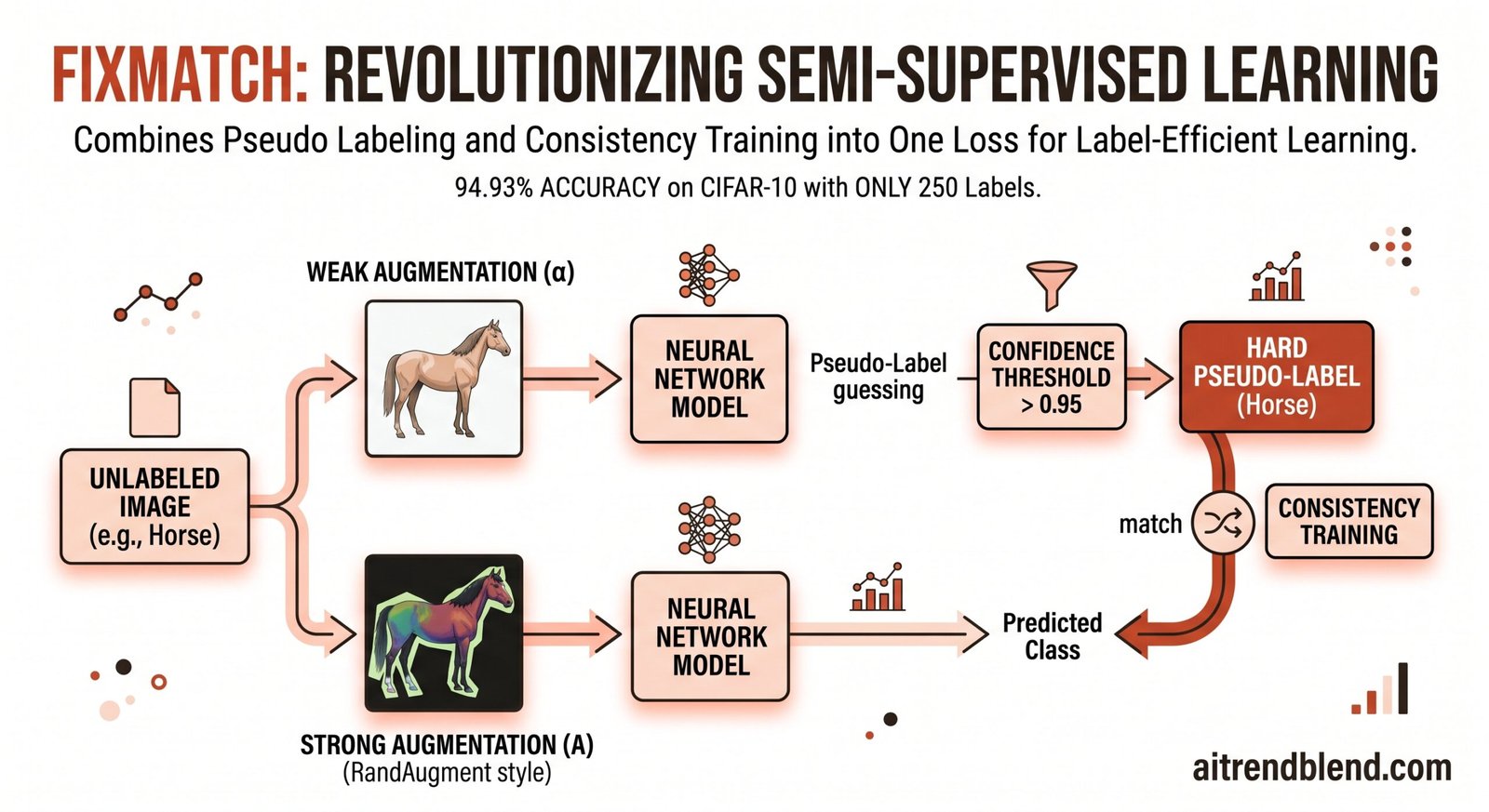
- A weakly augmented view of an unlabeled image produces the target label. A strongly augmented view of the same image has to match it, but only when the model is confident enough to clear a threshold.
- The authors’ ablation study found that the optimizer, the weight decay value, and the learning rate schedule mattered as much as the algorithm itself, a detail most semi supervised papers leave out.
- With just one labeled example per class, the right examples pushed accuracy above 80 percent, while the wrong examples never got the model to converge at all.
The problem FixMatch is actually solving
Deep networks are hungry. They get better with more data, and that pattern holds across vision, language, and just about every other domain researchers have thrown at them. The catch is that raw data is cheap while labeled data is not. Someone, or something, has to look at each image and decide what it is. In a lot of fields that someone is an expert, a radiologist reading a scan or a botanist sorting plant species, and that kind of labor does not scale the way GPU clusters do.
Semi supervised learning exists to soften that bottleneck. The pitch is straightforward. Use a small labeled set to teach the model what the categories look like, then let it learn additional structure from a much larger pool of unlabeled examples that cost nothing to collect. The hard part has always been turning “unlabeled data” into a usable training signal without the model quietly convincing itself of something false and reinforcing its own mistakes.
That difficulty produced a genuine arms race. Methods like MixMatch and ReMixMatch stacked averaging, sharpening, distribution alignment, and multiple loss terms on top of each other, and each addition bought a small accuracy gain at the cost of more hyperparameters to tune. FixMatch is the paper that asked whether most of that machinery was necessary in the first place, and the answer turned out to be no.
Two old ideas, one shared model
Consistency regularization rests on a simple assumption. A good model should give roughly the same answer for two different views of the same object. Perturb an image slightly, feed both versions through the network, and penalize the model when the predictions drift apart. Pseudo labeling takes a different route. It trusts the model’s own high confidence predictions enough to treat them as ground truth and trains against them directly.
Prior work usually picked one philosophy or blended them with extra machinery. FixMatch combines both in the plainest way its authors could manage. It generates a pseudo label from a weakly augmented image, keeps that label only if the model’s confidence clears a threshold, and then asks the model to reproduce that same label when it sees a heavily distorted version of the identical image. One model, one forward pass structure, two augmentation strengths, one loss.
How the loss function actually works
The supervised half of FixMatch is nothing unusual. It is standard cross entropy on weakly augmented labeled images.
The interesting part is the unlabeled term. For every unlabeled image, the model first sees a weakly augmented copy, meaning a flip and a small shift, and produces a predicted distribution over classes. The argmax of that distribution becomes the pseudo label, but only for images where the highest class probability exceeds a threshold set at 0.95 in nearly all of the paper’s experiments.
Here A denotes the strong augmentation, built from either RandAugment or CTAugment followed by Cutout, and q hat is the hardened one hot pseudo label. The total loss is just the supervised term plus the unlabeled term scaled by a fixed weight, set to 1 across almost every dataset in the paper. No annealing schedule, no separate warmup phase for the unlabeled weight, none of the extra scaffolding that ReMixMatch and UDA both needed.
Why weak for the label, strong for the prediction
This asymmetry is the actual novelty in the paper, more than the pseudo labeling or the consistency loss individually. The label guessing pass has to be reliable, so it runs on a barely altered image, just a flip and a small translation. The prediction pass that gets compared against that label runs on a heavily distorted version, cut out patches and aggressive color and geometric transforms drawn from RandAugment or CTAugment.
The authors tested what happens if you break that asymmetry. Swap in strong augmentation for the label guessing step and the model diverges early in training, since the pseudo labels themselves become unreliable garbage that the model then dutifully memorizes. Drop augmentation entirely from the label guessing step and the model overfits its own guesses. Use weak augmentation for both passes and accuracy peaks around 45 percent before collapsing to 12 percent as training continues. The gap between the two augmentation strengths is not a minor design choice, it is the mechanism that keeps the unlabeled loss from becoming an echo chamber.
What the benchmark numbers actually show
The authors reimplemented every baseline in a single shared codebase, following the evaluation protocol laid out in earlier work by Oliver and colleagues on realistic semi supervised evaluation, specifically so that architecture and training details would not quietly favor one method over another. That kind of apples to apples comparison is rarer in this literature than it should be.
| Method | CIFAR-10, 40 labels | CIFAR-10, 250 labels | CIFAR-100, 400 labels | SVHN, 40 labels |
|---|---|---|---|---|
| Pseudo Labeling | not reported | 49.78 error | not reported | not reported |
| Mean Teacher | not reported | 32.32 error | not reported | not reported |
| MixMatch | 47.54 error | 11.05 error | 67.61 error | 42.55 error |
| UDA | 29.05 error | 8.82 error | 59.28 error | 52.63 error |
| ReMixMatch | 19.10 error | 5.44 error | 44.28 error | 3.34 error |
| FixMatch, CTAugment | 11.39 error | 5.07 error | 49.95 error | 7.65 error |
All figures are error rates on held out test sets, averaged across five different folds of which examples were labeled, and lower is better. FixMatch wins on CIFAR-10 and SVHN outright and comes close on CIFAR-100, where ReMixMatch’s distribution alignment component still has an edge. When the authors bolted that same distribution alignment idea onto FixMatch, error on CIFAR-100 with 400 labels dropped to 40.14 percent, ahead of ReMixMatch’s own 44.28 percent, which suggests the gap was never about FixMatch’s core mechanism being weaker, just about which extras got included.
On STL-10, a dataset deliberately built with out of distribution images mixed into its unlabeled pool to stress test robustness, FixMatch again matches the previous state of the art from ReMixMatch. On ImageNet, using only 10 percent of the training set as labeled data, FixMatch reaches a 28.54 percent top-1 error rate, 2.68 points better than UDA under the same conditions.
The ablation study nobody else ran
Because FixMatch strips the method down to so few moving parts, the authors had room to run an unusually thorough ablation study, and some of the findings are more surprising than the headline accuracy numbers.
Sharpening versus thresholding
A softer version of pseudo labeling exists, called sharpening, where instead of taking a hard argmax you raise the predicted distribution to a temperature and renormalize it. MixMatch and ReMixMatch both use this. The authors tested it directly against hard thresholding and found sharpening added a hyperparameter, the temperature, without improving accuracy once a confidence threshold was already in place. The threshold alone, set to 0.95, gave the lowest error rate in their sweep, and pushing it up to 0.97 or 0.99 barely changed results.
The optimizer mattered more than expected
This is the part most semi supervised papers skip entirely. The authors swept SGD momentum values and found that setting momentum to 0.999 pushed error all the way up to 84.33 percent, essentially breaking training, while the default 0.9 gave 4.84 percent. They also tested Adam and found it consistently underperformed SGD with Nesterov momentum, and was far more sensitive to learning rate choice, with error jumping past 8 percent from a single learning rate change that barely moved SGD’s results.
Weight decay swings results by ten points
Choosing a weight decay value one order of magnitude off from optimal cost the model ten percentage points of accuracy or more in the low label regime. That is a bigger swing than the difference between FixMatch and its nearest semi supervised competitor. It is an uncomfortable finding for the field, since it means published comparisons between different semi supervised methods can be quietly distorted by how carefully each one’s supervised learning hyperparameters were tuned, independent of the actual semi supervised algorithm being tested.
What this means beyond the benchmark tables
The broader lesson of FixMatch is less about the specific numbers and more about method design discipline. Semi supervised learning had been trending toward increasingly elaborate pipelines, each new paper adding a term to fix a weakness introduced by the last paper’s fix. FixMatch is a reminder that combining two well understood ideas carefully, with attention paid to which augmentation feeds which branch of the loss, can outperform a stack of five techniques bolted together.
There is a practical upside too. Because the algorithm fits in a handful of lines and needs very few hyperparameters, it is genuinely usable outside a research lab. A team with a labeling budget for a few hundred images per class and a large pool of unlabeled data in the same domain, medical imaging being the example the authors themselves raise, has a real shot at applying this without a dedicated hyperparameter search team.
The authors are candid that this cuts both ways. The same low label efficiency that makes FixMatch useful for cheap, high value applications also makes more accurate few shot recognition systems easier to build for less benign purposes, identifying a person from very few reference images being their own example. That is not a reason to avoid the method, but it is a reason to think about deployment context before applying label efficient recognition at scale.
Honest limitations
FixMatch’s headline numbers come from a controlled academic setting. The labeled and unlabeled data are drawn from the exact same distribution in most experiments, which is a friendlier setup than most real deployments offer. STL-10 is the one benchmark here that includes out of distribution images in its unlabeled pool, and while FixMatch still performs well there, the paper does not stress test heavier distribution shift the way a deployed system might encounter.
The one label and four label per class results, while striking, carry very high variance. The authors report a standard deviation of 3.35 percent on the four label per class CIFAR-10 setting, compared with 0.33 percent at 25 labels per class, and different runs of the one label per class experiment landed anywhere between 48.58 percent and 85.32 percent accuracy depending purely on which ten images got sampled as labels. That is not a stable operating point, it is a demonstration of what is possible under favorable sampling, and practitioners should read it that way rather than as a guarantee.
Finally, the ablation study itself, while unusually thorough, was run almost entirely on a single 250 label CIFAR-10 split for practical reasons. The authors are transparent about this scope limit, but it does mean some of the fine grained sensitivity findings, like the exact optimal weight decay value, may not transfer cleanly to a different dataset or a different label budget without re tuning.
Complete PyTorch implementation
The following is a full, runnable implementation of the FixMatch training loop, including the weak and strong augmentation split, the confidence threshold, the combined loss, and a smoke test on random dummy data so you can confirm the pipeline runs before pointing it at a real dataset.
# A minimal, runnable FixMatch implementation for demonstration and smoke testing.
import torch
import torch.nn as nn
import torch.nn.functional as F
from torch.utils.data import DataLoader, TensorDataset
# —- A small Wide ResNet style backbone, simplified for readability —-
class BasicBlock(nn.Module):
def __init__(self, in_ch, out_ch, stride=1):
super().__init__()
self.bn1 = nn.BatchNorm2d(in_ch)
self.conv1 = nn.Conv2d(in_ch, out_ch, 3, stride=stride, padding=1, bias=False)
self.bn2 = nn.BatchNorm2d(out_ch)
self.conv2 = nn.Conv2d(out_ch, out_ch, 3, stride=1, padding=1, bias=False)
self.shortcut = None
if stride != 1 or in_ch != out_ch:
self.shortcut = nn.Conv2d(in_ch, out_ch, 1, stride=stride, bias=False)
def forward(self, x):
out = F.relu(self.bn1(x))
shortcut = self.shortcut(out) if self.shortcut is not None else x
out = self.conv1(out)
out = self.conv2(F.relu(self.bn2(out)))
return out + shortcut
class WideResNet(nn.Module):
def __init__(self, num_classes=10, widen=2, depth_blocks=4):
super().__init__()
widths = [16, 16 * widen, 32 * widen, 64 * widen]
self.stem = nn.Conv2d(3, widths[0], 3, padding=1, bias=False)
layers = []
in_ch = widths[0]
for stage, out_ch in enumerate(widths[1:]):
stride = 1 if stage == 0 else 2
for b in range(depth_blocks):
layers.append(BasicBlock(in_ch, out_ch, stride if b == 0 else 1))
in_ch = out_ch
self.blocks = nn.Sequential(*layers)
self.bn_final = nn.BatchNorm2d(in_ch)
self.fc = nn.Linear(in_ch, num_classes)
def forward(self, x):
x = self.stem(x)
x = self.blocks(x)
x = F.relu(self.bn_final(x))
x = F.adaptive_avg_pool2d(x, 1).flatten(1)
return self.fc(x)
# —- Weak and strong augmentation stand ins —-
# In a real run, weak_augment is flip and shift, strong_augment is RandAugment
# or CTAugment followed by Cutout. These are simplified placeholders that keep
# the same interface so the training loop below is fully runnable end to end.
def weak_augment(images):
if torch.rand(1).item() < 0.5:
images = torch.flip(images, dims=[3])
shift = torch.randint(-2, 3, (2,))
images = torch.roll(images, shifts=(shift[0].item(), shift[1].item()), dims=(2, 3))
return images
def strong_augment(images):
noise = torch.randn_like(images) * 0.3
images = torch.clamp(images + noise, -3.0, 3.0)
# Cutout style masking of a random square patch
b, c, h, w = images.shape
size = max(1, h // 4)
cy, cx = torch.randint(0, h, (1,)).item(), torch.randint(0, w, (1,)).item()
y0, y1 = max(0, cy – size), min(h, cy + size)
x0, x1 = max(0, cx – size), min(w, cx + size)
images[:, :, y0:y1, x0:x1] = 0.0
return images
# —- FixMatch loss, matching equations 3 and 4 of the paper —-
def fixmatch_loss(model, labeled_images, labels, unlabeled_images, tau=0.95, lambda_u=1.0):
# Supervised term, weak augmentation only
sup_logits = model(weak_augment(labeled_images))
sup_loss = F.cross_entropy(sup_logits, labels)
# Pseudo label from the weakly augmented unlabeled batch, no gradient needed
with torch.no_grad():
weak_logits = model(weak_augment(unlabeled_images))
probs = F.softmax(weak_logits, dim=1)
max_probs, pseudo_labels = probs.max(dim=1)
mask = (max_probs >= tau).float()
# Prediction from the strongly augmented unlabeled batch, gradients flow here
strong_logits = model(strong_augment(unlabeled_images))
unsup_loss_per_example = F.cross_entropy(strong_logits, pseudo_labels, reduction=‘none’)
unsup_loss = (unsup_loss_per_example * mask).mean()
total_loss = sup_loss + lambda_u * unsup_loss
return total_loss, sup_loss.item(), unsup_loss.item(), mask.mean().item()
# —- Training loop —-
def train(model, labeled_loader, unlabeled_loader, steps=200, lr=0.03, momentum=0.9, weight_decay=0.0005):
optimizer = torch.optim.SGD(model.parameters(), lr=lr, momentum=momentum, nesterov=True, weight_decay=weight_decay)
scheduler = torch.optim.lr_scheduler.CosineAnnealingLR(optimizer, T_max=steps)
labeled_iter = iter(labeled_loader)
unlabeled_iter = iter(unlabeled_loader)
model.train()
for step in range(steps):
try:
lx, ly = next(labeled_iter)
except StopIteration:
labeled_iter = iter(labeled_loader)
lx, ly = next(labeled_iter)
try:
(ux,) = next(unlabeled_iter)
except StopIteration:
unlabeled_iter = iter(unlabeled_loader)
(ux,) = next(unlabeled_iter)
optimizer.zero_grad()
loss, sup, unsup, mask_rate = fixmatch_loss(model, lx, ly, ux)
loss.backward()
optimizer.step()
scheduler.step()
if step % 50 == 0:
print(f“step {step} loss {loss.item():.4f} sup {sup:.4f} unsup {unsup:.4f} mask rate {mask_rate:.2f}”)
# —- Evaluation function —-
def evaluate(model, loader):
model.eval()
correct, total = 0, 0
with torch.no_grad():
for x, y in loader:
preds = model(x).argmax(dim=1)
correct += (preds == y).sum().item()
total += y.size(0)
model.train()
return correct / total
# —- Smoke test on random dummy data —-
if __name__ == “__main__”:
torch.manual_seed(0)
num_classes = 10
model = WideResNet(num_classes=num_classes, widen=2, depth_blocks=2)
# Dummy labeled set, 40 images, four per class in spirit only
labeled_x = torch.randn(40, 3, 32, 32)
labeled_y = torch.randint(0, num_classes, (40,))
labeled_ds = TensorDataset(labeled_x, labeled_y)
labeled_loader = DataLoader(labeled_ds, batch_size=8, shuffle=True)
# Dummy unlabeled set, larger pool, no labels used
unlabeled_x = torch.randn(200, 3, 32, 32)
unlabeled_ds = TensorDataset(unlabeled_x)
unlabeled_loader = DataLoader(unlabeled_ds, batch_size=8 * 7, shuffle=True)
# Dummy test set for the evaluation function
test_x = torch.randn(50, 3, 32, 32)
test_y = torch.randint(0, num_classes, (50,))
test_loader = DataLoader(TensorDataset(test_x, test_y), batch_size=10)
train(model, labeled_loader, unlabeled_loader, steps=20)
acc = evaluate(model, test_loader)
print(f“smoke test complete, dummy accuracy {acc:.2f}”)
Full conclusion
FixMatch earns its place in this conversation not because it introduces a clever new mechanism nobody had seen before, but because it demonstrates how much of the recent semi supervised learning literature had been solving problems its own added complexity created. Pseudo labeling and consistency regularization are both old ideas, dating back decades in one case, yet nobody had combined them with this particular weak strong augmentation split and let the confidence threshold do the scheduling work that other methods handled with manual annealing.
The conceptual shift worth sitting with is that the paper’s real contribution is subtractive. Every recent competitor added a component, sharpening, distribution alignment, multiple augmented views averaged together, and FixMatch instead asked which of those were load bearing and which were compensating for something the augmentation split already handled. The ablation study answers that question directly, and the honest surprise is that basic training choices like the optimizer and weight decay moved the needle as much as any semi supervised specific trick.
Transferability is where this gets genuinely useful outside the CIFAR benchmarks. The core loss function does not care what the input modality is, only that a meaningful notion of weak and strong perturbation exists for it. The paper’s own appendix experiments with datatype agnostic alternatives like MixUp and virtual adversarial training in place of image specific augmentation, and both worked, which suggests the recipe generalizes past vision into any domain with a workable augmentation strategy, text and speech included given the domain specific augmentation methods already cited in the paper.
The honest remaining limitations matter as much as the wins. High variance at the extreme low label counts, a controlled academic setting where labeled and unlabeled data mostly share a distribution, and an ablation study run predominantly on one dataset all mean the specific hyperparameters here are a starting point, not a universal setting. Anyone applying this to a new domain should expect to re run at least the confidence threshold and weight decay sweeps rather than copying the CIFAR-10 values wholesale.
Where this leaves the field is with a genuinely lower barrier to entry. A method that fits in a page of loss code, needs one confidence threshold and one loss weight as its main new hyperparameters, and still beats far more elaborate predecessors changes who gets to experiment with semi supervised learning in the first place. That, more than any single accuracy number in the tables above, is the lasting contribution here.
Go deeper on the source material
Read the full paper for the complete ablation tables, the ImageNet and STL-10 details, and the barely supervised learning appendix.
Read the paper on arXiv View the official codeFrequently asked questions
What does FixMatch actually stand for as a method?
It is not an acronym. The name reflects the method fixing a pseudo label from a weakly augmented image and matching a strongly augmented prediction against it, combining pseudo labeling with consistency regularization into one loss.
How few labels can FixMatch work with?
The paper reports 88.61 percent accuracy on CIFAR-10 with only 40 labeled images total, four per class. In a further experiment with just one label per class, accuracy ranged from 48.58 percent to 85.32 percent depending entirely on which single example represented each class.
What is the role of the confidence threshold?
It decides which pseudo labels are trustworthy enough to train against. A predicted probability has to exceed 0.95 before its pseudo label counts toward the unlabeled loss, which the authors found more effective than softening low confidence predictions through sharpening.
Does FixMatch require a special network architecture?
No. The paper uses standard Wide ResNet architectures for CIFAR-10, CIFAR-100, SVHN, and STL-10, and a standard ResNet-50 for the ImageNet experiments. The method is a training recipe, not an architecture change.
Why does the optimizer choice matter so much in this paper?
The authors found that momentum, weight decay, and learning rate schedule choices could shift error rates by ten percentage points or more, sometimes more than the difference between competing semi supervised algorithms. They argue these basic supervised learning factors are underreported elsewhere in the field.
Can FixMatch be applied outside image classification?
The paper’s appendix tests datatype agnostic alternatives to image augmentation, including MixUp and virtual adversarial training, and both produced reasonable results, suggesting the core loss transfers to other modalities that have a workable notion of weak and strong perturbation.
Related reading
This analysis is based on the published paper and an independent evaluation of its claims.