
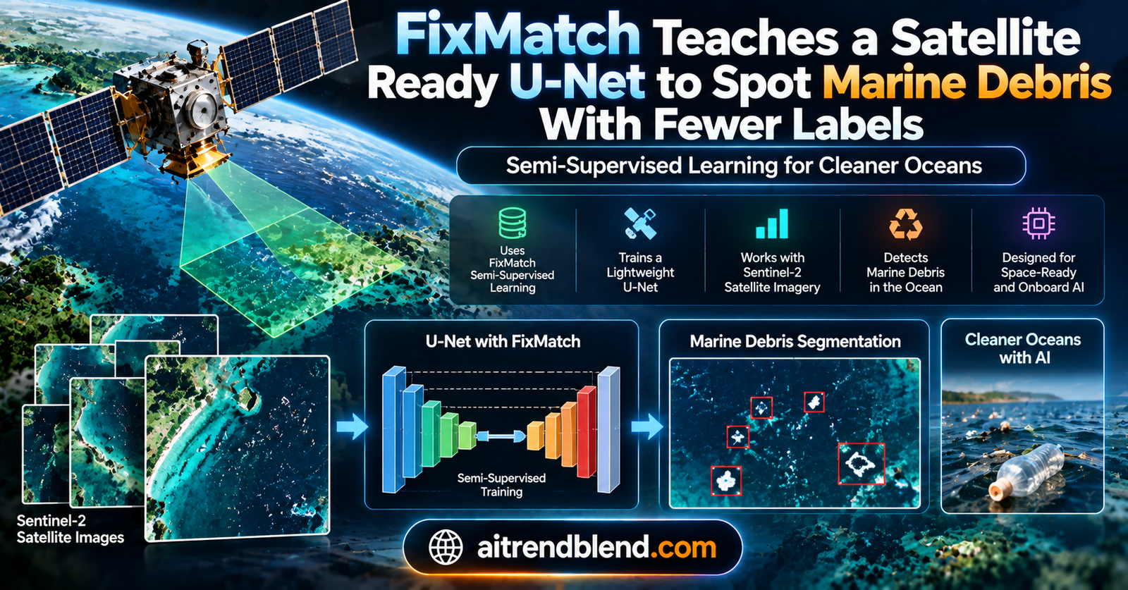
Key points
- The thesis adapts FixMatch, a popular semi supervised learning method built for image classification, to pixel level semantic segmentation of marine anomalies in Sentinel 2 imagery.
- With 30 percent or less of the training labels available, the semi supervised model beats a fully supervised model trained on the same labeled subset by an average of 6.5 percent test mIoU.
- That advantage reverses once 40 percent or more of the labels are available, where the fully supervised model pulls ahead by an average of 3 percent test mIoU.
- Every model uses a compact U-Net with 841,099 parameters and a 3.25 megabyte weight file, sized deliberately to run on space rated satellite hardware.
- The author proposes two competing explanations for why the semi supervised advantage fades as labeled data grows, and neither one is fully confirmed.
Why satellites still cannot decide for themselves
Earth observation satellites capture an enormous amount of imagery that nobody looks at directly. A satellite photographs the ocean, stores the image, and waits until it passes over a ground station to downlink everything it recorded. Most of what gets transmitted down that narrow radio link is featureless open water. If the satellite could recognize which images actually contain something worth reporting, marine debris, an oil slick, a vessel behaving suspiciously, it could send only the useful fraction and save the rest of its downlink budget for imagery that matters. That idea, running inference onboard the spacecraft rather than waiting for ground processing, is the practical motivation running through the entire thesis by Luca Marini, supervised by researchers from the European Space Agency, AI Sweden and TU Delft.
The obstacle is not model design so much as data. Semantic segmentation, the task of labeling every pixel of an image with a class, needs pixel accurate ground truth to train on, and pixel accurate ground truth for marine anomalies is slow and expensive to produce. An annotator has to squint at a multispectral composite and decide where exactly a barely visible ribbon of Sargassum algae ends and open water begins. The MARIDA dataset used throughout this work, a collection of Sentinel 2 patches assembled specifically for marine debris research, only has 837,377 labeled pixels total across its training, validation and test splits, and most of those pixels are ordinary water rather than anomalies. That scarcity is exactly the situation semi supervised learning was built for. Use the small labeled set for direct supervision, and let a much larger pool of unlabeled imagery contribute a second training signal.
Turning FixMatch from a classifier into a pixel labeler
FixMatch itself is not new. It became one of the most widely used semi supervised learning recipes for image classification because it combines two established ideas, pseudo labeling and consistency regularization, into a method simple enough to implement in an afternoon. Feed an unlabeled image through the model after a weak augmentation, such as a flip. If the model is highly confident about its prediction, treat that prediction as a pseudo label. Then feed a strongly augmented version of the same image through the model again and train it to reproduce that pseudo label. The logic is that a model confident enough about an easy view of an image should stay confident under a harder, more distorted view, and forcing that consistency teaches the model something useful even without a human supplied answer.
Applying that logic to image classification is straightforward because a rotated photograph of a ship is still a photograph of a ship, the label does not change when the geometry changes. Semantic segmentation breaks that assumption. Rotate or shear a satellite image and the pixel level label map has to rotate and shear along with it, or the augmented label will point at the wrong location entirely. The thesis works through this adaptation carefully, applying every geometric augmentation to the pseudo label map in lockstep with the image, while reserving color based augmentations such as solarization and sharpness adjustment for cases where the label map does not need to move at all.
Two loss terms doing different jobs
The training objective ends up as two separate pieces added together. The supervised term only ever sees labeled pixels, using a focal loss rather than plain cross entropy because the dataset is severely imbalanced. Water pixels outnumber marine debris pixels by roughly two hundred to one after the author collapses the original fifteen MARIDA categories down to five practical classes, Marine Debris, Algae or Organic Material, Ship, Cloud and Water. Focal loss down weights the easy, already well classified water pixels so the model keeps paying attention to the rare and harder classes instead of coasting on background accuracy.
The unsupervised term only ever touches unlabeled pixels, and only the ones where the model’s pseudo label prediction clears a confidence threshold τ. Here the author uses ordinary cross entropy rather than focal loss, reasoning that once a pixel has already survived a high confidence filter, there is no remaining need to further discount it. A separate hyperparameter μ controls how many unlabeled images get pulled into each training step relative to labeled ones, set to five throughout the experiments to keep GPU memory in check.
A U-Net small enough to fly
Every model trained in this thesis shares the same architecture, a standard U-Net with skip connections between its downsampling and upsampling paths, sized down to 841,099 parameters. That is a deliberately small model. The author benchmarks it at 2.07 GFLOPs per inference on an eleven channel, 256 by 256 pixel patch and reports a saved weight file of 3.25 megabytes. Those numbers are measured against a specific piece of space rated hardware, the Unibap SpaceCloud iX5-106, whose onboard GPU offers 87 GFLOPS of compute and 240 gigabytes of storage. A 3.25 megabyte model file against 240 gigabytes of available storage is not a tight fit at all, which is the point. The architecture choice was constrained from the start by what a satellite can actually carry and run, not by what produces the best possible benchmark score on a workstation.
What actually happened when labels got scarce
The main experiment trains matched pairs of models, one fully supervised and one semi supervised, at nine different labeled data percentages from 5 percent up to 80 percent of the MARIDA training set, always using the identical labeled subset for both models in a pair so the comparison is fair. The unlabeled counterpart in the semi supervised setup is simply the rest of the training set treated as if it carried no labels at all.
| Labeled data | Fully supervised test mIoU | Semi supervised test mIoU | Difference |
|---|---|---|---|
| 5 percent | 0.46 | 0.57 | +11 |
| 10 percent | 0.61 | 0.65 | +4 |
| 20 percent | 0.72 | 0.80 | +8 |
| 30 percent | 0.86 | 0.89 | +3 |
| 40 percent | 0.89 | 0.86 | -3 |
| 50 percent | 0.86 | 0.82 | -4 |
| 60 percent | 0.88 | 0.90 | +2 |
| 70 percent | 0.88 | 0.84 | -4 |
| 80 percent | 0.91 | 0.90 | -1 |
Below 30 percent labeled data, the semi supervised model wins or matches its fully supervised counterpart every time, averaging 6.5 percent higher test mIoU across that range. Past 40 percent, the trend flips in four of five cases, with the exception at 60 percent, and the fully supervised model averages 3 percent ahead when that outlier is excluded. The two curves converge as more labels become available, which is exactly what intuition would predict, a model that already has enough labeled examples has less to gain from a noisy secondary signal.
Two competing explanations, neither fully proven
The author offers two hypotheses for why the advantage reverses, and is careful not to claim either one is confirmed. The first is that once the labeled set alone already produces strong performance, only the easiest, most obviously classified pseudo labels clear the confidence threshold, meaning the unsupervised loss term stops contributing anything the model did not already know. The second hypothesis is structural rather than behavioral. In this experimental setup, every image belongs entirely to either the labeled pool or the unlabeled pool. As the labeled percentage climbs, the unlabeled pool necessarily shrinks, so there is simply less raw material left for the consistency regularization term to learn from, independent of how confident the pseudo labels are. Both explanations are plausible and the thesis does not run the additional experiments that would be needed to separate them.
A discovery that came from watching the wrong metric
One of the more interesting findings shows up almost as a side effect. At 30 percent and 70 percent labeled data, the fully supervised and semi supervised models land on essentially identical validation mIoU scores, yet their test set performance diverges noticeably. Digging into the training curves, the author finds that the model with the lower validation loss at that point, not the higher validation mIoU, is consistently the one that generalizes better to the test set. mIoU and loss usually move together, so when they do not, the loss curve turns out to be the more trustworthy signal. It is a small methodological note buried in a larger thesis, but it is a genuinely useful piece of practical advice for anyone tuning a segmentation model under a tight label budget.
What the confidence threshold experiments taught the author
Before running the headline comparison, the author swept the pseudo label confidence threshold τ across 0.5, 0.6, 0.7, 0.8 and 0.9, training on just 10 percent labeled data to keep the search affordable. A threshold of 0.9 produced the best result on both validation and test sets, reaching 0.63 test mIoU against scores in the mid 0.50s for the lower thresholds. The explanation lines up with the original FixMatch paper’s own finding, a low threshold lets in more pseudo labels but also more wrong ones, and early in training, before the model has learned much, wrong pseudo labels can compound into a feedback loop sometimes called confirmation bias, where the model becomes increasingly confident about its own mistakes.
A separate check compared cross entropy against focal loss specifically for the unsupervised loss term, motivated by the concern that focal loss might suppress the signal from exactly the high confidence pseudo labels the threshold was designed to keep. The two options landed within 0.001 mIoU of each other, close enough that the author treats the choice as essentially inconsequential for this dataset, though the underlying loss curves showed some divergence during the earliest and latest training epochs that the thesis flags without fully resolving.
Where the visual predictions get interesting
Averaged scores hide individual failures, so the author picked apart which classes swung the most across the labeled data percentages and looked directly at the predicted segmentation maps for Cloud and Marine Debris, the two classes with the highest variance in performance gap. For Cloud, the semi supervised model’s best showing, a 24 percent test mIoU improvement, came at the lowest labeled data setting of 5 percent, where it caught clouds the fully supervised model missed outright. Its worst showing for Cloud, a 17 percent drop at 70 percent labeled data, traced back to just three test patches out of roughly forty five containing cloud pixels, and one of those three had what the author calls unusual ground truth labeling, with pixels that visually look like water labeled as cloud in the reference annotation. A small number of mislabeled test patches can swing an aggregate score meaningfully when a class is otherwise rare in the test set.
Honest limitations
The thesis is candid about where its conclusions do not extend. The MARIDA patches used throughout are atmospherically corrected, co registered across bands, and georeferenced, none of which is guaranteed for raw data actually available onboard a satellite before ground processing. The author is explicit that this is an optimistic assumption baked into the entire experimental setup, and that the georeferenced coordinate transmission concept described for reducing downlink usage depends on it holding true. Several of the five classes rest on very few labeled pixels, Marine Debris totals only 3,399 labeled pixels across the entire dataset, which limits how confidently these results generalize to debris in other regions of the world with different lighting, water color and debris composition. The MARIDA dataset also contains no land labeled pixels at all, so a model trained on it has no learned concept of land and would likely misclassify coastal or inland scenes as some combination of its five water adjacent categories. Finally, none of the models were actually run on space rated hardware. The GFLOPs and parameter counts were computed on paper against published specifications, not measured through an onboard deployment test.
Why this matters beyond one satellite mission
Step outside the specific onboard AI framing and this thesis is really a case study in a question that comes up constantly in applied machine learning. When annotation is the bottleneck rather than compute or model capacity, does semi supervised learning actually deliver on its promise, or is it a technique that only looks good in papers with generous unlabeled data budgets. The honest answer this work arrives at is conditional rather than universal. Semi supervised learning helped substantially in the regime where most real world teams actually operate, under 30 percent of the data they would ideally want labeled, and stopped helping once the labeled budget crossed a threshold specific to this dataset and task. That is a more useful and more believable finding than a blanket claim that semi supervised learning always wins, because it gives a practitioner a concrete signal for when to bother with the added complexity of pseudo labeling and consistency regularization and when a straightforward supervised baseline is good enough.
The onboard AI angle also has implications that reach past marine debris specifically. Any Earth observation task built around detecting a rare event in a sea of uninteresting imagery, wildfire smoke, illegal deforestation, oil spills, faces the identical bottleneck of expensive pixel level labels against an ocean of unlabeled acquisitions. A validated recipe for squeezing useful signal out of that unlabeled majority, even a conditional one, is a transferable piece of engineering knowledge for the wider remote sensing field, not just for the specific five classes studied here.
PyTorch implementation
The following code reconstructs the core pieces described in the thesis, the compact U-Net, the focal loss used for the supervised term, and the FixMatch style supervised and unsupervised losses adapted for pixel level segmentation with an ignore label for unlabeled pixels. It runs as a self contained smoke test on synthetic data to confirm the shapes and loss computations before swapping in real MARIDA patches.
# fixmatch_segmentation.py
# Reconstructed implementation of FixMatch for Semantic Segmentation,
# adapted for marine anomaly detection on multispectral satellite patches.
# Reference: Marini, L. "Semi-supervised learning for marine anomaly
# detection on board satellites." Masters thesis, KTH, 2023.

import torch
import torch.nn as nn
import torch.nn.functional as F

IGNORE_INDEX = -1
NUM_CLASSES = 5  # Marine Debris, Algae/Organic Material, Ship, Cloud, Water


class ConvBlock(nn.Module):
    def __init__(self, in_ch: int, out_ch: int):
        super().__init__()
        self.block = nn.Sequential(
            nn.Conv2d(in_ch, out_ch, kernel_size=3, padding=1),
            nn.BatchNorm2d(out_ch),
            nn.ReLU(inplace=True),
            nn.Conv2d(out_ch, out_ch, kernel_size=3, padding=1),
            nn.BatchNorm2d(out_ch),
            nn.ReLU(inplace=True),
        )

    def forward(self, x):
        return self.block(x)


class CompactUNet(nn.Module):
    """A downsized U-Net with a narrow channel width, matched to the
    841,099 parameter, 2.07 GFLOP footprint reported in the thesis
    for an 11 channel, 256x256 input patch."""

    def __init__(self, in_channels: int = 11, num_classes: int = NUM_CLASSES, base_width: int = 24):
        super().__init__()
        w = base_width
        self.enc1 = ConvBlock(in_channels, w)
        self.enc2 = ConvBlock(w, w * 2)
        self.enc3 = ConvBlock(w * 2, w * 4)
        self.pool = nn.MaxPool2d(2)

        self.bottleneck = ConvBlock(w * 4, w * 8)

        self.up3 = nn.Upsample(scale_factor=2, mode="bilinear", align_corners=True)
        self.dec3 = ConvBlock(w * 8 + w * 4, w * 4)
        self.up2 = nn.Upsample(scale_factor=2, mode="bilinear", align_corners=True)
        self.dec2 = ConvBlock(w * 4 + w * 2, w * 2)
        self.up1 = nn.Upsample(scale_factor=2, mode="bilinear", align_corners=True)
        self.dec1 = ConvBlock(w * 2 + w, w)

        self.head = nn.Conv2d(w, num_classes, kernel_size=1)

    def forward(self, x):
        e1 = self.enc1(x)
        e2 = self.enc2(self.pool(e1))
        e3 = self.enc3(self.pool(e2))
        b = self.bottleneck(self.pool(e3))

        d3 = self.dec3(torch.cat([self.up3(b), e3], dim=1))
        d2 = self.dec2(torch.cat([self.up2(d3), e2], dim=1))
        d1 = self.dec1(torch.cat([self.up1(d2), e1], dim=1))

        return self.head(d1)  # (batch, num_classes, H, W) logits


class FocalLoss(nn.Module):
    """Equation 3.8. Down-weights easy, already well classified
    pixels so training keeps attending to rare classes such as
    Marine Debris, which make up under half a percent of labeled
    pixels in the grouped five class MARIDA setup."""

    def __init__(self, gamma: float = 2.0, alpha: torch.Tensor = None, ignore_index: int = IGNORE_INDEX):
        super().__init__()
        self.gamma = gamma
        self.alpha = alpha
        self.ignore_index = ignore_index

    def forward(self, logits: torch.Tensor, targets: torch.Tensor):
        # logits: (batch, classes, H, W), targets: (batch, H, W) with -1 for unlabeled
        log_probs = F.log_softmax(logits, dim=1)
        probs = log_probs.exp()

        valid = targets != self.ignore_index
        safe_targets = targets.clone()
        safe_targets[~valid] = 0  # placeholder, masked out below

        pt = probs.gather(1, safe_targets.unsqueeze(1)).squeeze(1)
        log_pt = log_probs.gather(1, safe_targets.unsqueeze(1)).squeeze(1)

        if self.alpha is not None:
            alpha_t = self.alpha.to(logits.device)[safe_targets]
        else:
            alpha_t = 1.0

        loss = -alpha_t * (1 - pt).pow(self.gamma) * log_pt
        loss = loss[valid]
        return loss.mean() if loss.numel() > 0 else torch.tensor(0.0, device=logits.device)


def supervised_loss(model: nn.Module, images: torch.Tensor, labels: torch.Tensor, focal: FocalLoss):
    """Equation 3.9. Weak augmentation is assumed to already have
    been applied to images and labels together before this call."""
    logits = model(images)
    return focal(logits, labels)


def unsupervised_loss(
    model: nn.Module,
    weak_images: torch.Tensor,
    strong_images: torch.Tensor,
    threshold: float = 0.9,
):
    """Equation 3.10. Generates pseudo labels from a weakly augmented
    view, keeps only pixels whose confidence clears the threshold,
    then trains the strongly augmented view to match them."""
    with torch.no_grad():
        weak_logits = model(weak_images)
        weak_probs = F.softmax(weak_logits, dim=1)
        confidence, pseudo_labels = weak_probs.max(dim=1)
        keep_mask = confidence >= threshold

    strong_logits = model(strong_images)
    per_pixel_ce = F.cross_entropy(strong_logits, pseudo_labels, reduction="none")

    if keep_mask.sum() == 0:
        return torch.tensor(0.0, device=strong_images.device), 0.0

    masked_loss = (per_pixel_ce * keep_mask).sum() / keep_mask.sum().clamp_min(1)
    kept_fraction = keep_mask.float().mean().item()
    return masked_loss, kept_fraction


def fixmatch_segmentation_loss(
    model: nn.Module,
    labeled_images: torch.Tensor,
    labeled_targets: torch.Tensor,
    unlabeled_weak: torch.Tensor,
    unlabeled_strong: torch.Tensor,
    focal: FocalLoss,
    lambda_coeff: float = 1.0,
    threshold: float = 0.9,
):
    """L = Ls + lambda * Lu, the total FixMatch for Semantic
    Segmentation objective."""
    sup_loss = supervised_loss(model, labeled_images, labeled_targets, focal)
    unsup_loss, kept_fraction = unsupervised_loss(model, unlabeled_weak, unlabeled_strong, threshold)
    total = sup_loss + lambda_coeff * unsup_loss
    return total, {"sup": sup_loss.item(), "unsup": unsup_loss.item(), "kept_fraction": kept_fraction}


@torch.no_grad()
def mean_iou(logits: torch.Tensor, targets: torch.Tensor, num_classes: int = NUM_CLASSES, ignore_index: int = IGNORE_INDEX):
    """Equations 3.15 and 3.16. Mean intersection over union across
    classes, ignoring unlabeled pixels."""
    preds = logits.argmax(dim=1)
    valid = targets != ignore_index
    ious = []
    for c in range(num_classes):
        pred_c = (preds == c) & valid
        true_c = (targets == c) & valid
        intersection = (pred_c & true_c).sum().item()
        union = (pred_c | true_c).sum().item()
        if union > 0:
            ious.append(intersection / union)
    return sum(ious) / len(ious) if ious else 0.0


def train_step(model, optimizer, labeled_batch, unlabeled_batch, focal, lambda_coeff=1.0, threshold=0.9):
    model.train()
    optimizer.zero_grad()

    labeled_images, labeled_targets = labeled_batch
    unlabeled_weak, unlabeled_strong = unlabeled_batch

    loss, parts = fixmatch_segmentation_loss(
        model, labeled_images, labeled_targets,
        unlabeled_weak, unlabeled_strong, focal,
        lambda_coeff=lambda_coeff, threshold=threshold,
    )
    loss.backward()
    optimizer.step()
    return loss.item(), parts


def smoke_test():
    """Runs one training step and one mIoU evaluation on random
    dummy data shaped like an 11 band, 256x256 MARIDA patch."""
    torch.manual_seed(0)
    batch, channels, height, width = 2, 11, 256, 256

    labeled_images = torch.randn(batch, channels, height, width)
    labeled_targets = torch.randint(-1, NUM_CLASSES, (batch, height, width))

    unlabeled_weak = torch.randn(batch, channels, height, width)
    unlabeled_strong = torch.randn(batch, channels, height, width)

    # class frequencies from Table 3.1, used to weight the focal loss
    class_pixel_fractions = torch.tensor([0.0041, 0.0072, 0.0069, 0.1402, 0.8416])
    alpha = (1.0 / class_pixel_fractions)
    alpha = alpha / alpha.sum()

    model = CompactUNet(in_channels=channels, num_classes=NUM_CLASSES, base_width=16)
    focal = FocalLoss(gamma=2.0, alpha=alpha)
    optimizer = torch.optim.Adam(model.parameters(), lr=2e-4)

    loss, parts = train_step(
        model, optimizer,
        (labeled_images, labeled_targets),
        (unlabeled_weak, unlabeled_strong),
        focal, lambda_coeff=1.0, threshold=0.9,
    )
    print(f"total loss {loss:.4f}")
    for name, value in parts.items():
        print(f"  {name}: {value}")

    with torch.no_grad():
        eval_logits = model(labeled_images)
    score = mean_iou(eval_logits, labeled_targets, num_classes=NUM_CLASSES)
    print(f"smoke test mIoU on random data {score:.4f}")

    assert torch.isfinite(torch.tensor(loss)), "loss is not finite"
    print("smoke test passed")


if __name__ == "__main__":
    smoke_test()
Conclusion
The core achievement of this thesis is a working demonstration that FixMatch, originally built and tuned for classifying natural photographs, can be adapted into a functioning semantic segmentation pipeline for a genuinely difficult remote sensing problem, weakly labeled multispectral satellite patches with severe class imbalance. That adaptation was not trivial. Getting the geometric augmentations to move labels and images in lockstep, choosing focal loss for the supervised term while keeping cross entropy for the confident pseudo labels, and tuning the confidence threshold specifically for this label scarce regime all required deliberate engineering choices rather than a direct copy of the original recipe.
The conceptual shift worth carrying forward is the conditional nature of the result. Semi supervised learning is often pitched as a free performance boost, add unlabeled data and get better scores. This thesis shows a more nuanced and more useful reality: the boost is real and substantial exactly when labels are genuinely scarce, and it fades, sometimes reverses, once labels stop being the binding constraint. That is a finding with obvious transferability to other remote sensing tasks facing the identical rare event, abundant background imagery problem, wildfire smoke detection, illegal fishing vessel identification, deforestation monitoring, anywhere a satellite generates far more imagery than any team can afford to label by hand.
What remains genuinely open is everything downstream of the model itself. The author is upfront that none of this was tested on actual space rated hardware, and that the atmospherically corrected, co registered, georeferenced version of the data used throughout is a best case scenario unlikely to match what a satellite has access to before ground processing. Closing that gap, running the compact U-Net on hardware like the Unibap SpaceCloud iX5-106 under realistic power and radiation constraints, and testing against imagery that has not been through the MARIDA preprocessing pipeline, is where this work would need to go before onboard deployment becomes more than a plausible idea on paper.
The two open hypotheses for why the semi supervised advantage fades are also worth taking seriously as a research gap rather than a settled explanation. Distinguishing between a pseudo label confidence ceiling and a shrinking unlabeled pool would need a deliberately designed follow up experiment, perhaps one that holds the size of the unlabeled pool fixed while varying only the labeled percentage, something this thesis’s fixed dataset budget did not allow for.
Even with those gaps, the practical takeaway holds up. Teams working with scarce, expensive labels and an abundance of unlabeled imagery now have a reasonably well documented recipe, including public code, for testing whether semi supervised segmentation will actually help their specific problem before committing to a full pseudo labeling pipeline. Given how common the labeled data bottleneck is across remote sensing applications, that is a useful contribution whether or not the onboard satellite angle ever becomes standard practice.
Frequently asked questions
What is FixMatch and why does it need adapting for satellite imagery
FixMatch is a semi supervised learning method that generates pseudo labels from confident predictions on weakly augmented unlabeled images, then trains the model to reproduce those same pseudo labels on strongly augmented versions of the same images. It was originally designed for whole image classification, where a label does not change under geometric transformations. Semantic segmentation of satellite imagery requires every pixel to carry its own label, so any geometric augmentation applied to the image must be applied identically to its label map, which the original FixMatch recipe does not handle.
Does semi supervised learning always beat fully supervised training
No. In this thesis it only wins when 30 percent or less of the available training labels are used. Once 40 percent or more of the labels are available, fully supervised training pulls ahead in most of the tested cases. The two approaches converge as more labeled data becomes available.
What is the MARIDA dataset
MARIDA, short for Marine Debris Archive, is a dataset of multispectral Sentinel 2 satellite patches labeled for marine anomalies including marine debris, ships, algae and clouds. It is weakly labeled, meaning most pixels in each patch have no assigned class, and this thesis groups its original fifteen categories into five practical classes for training.
Was this model actually run on satellite hardware
No. The model’s parameter count and computational cost were calculated against the published specifications of a specific space rated processor, the Unibap SpaceCloud iX5-106, but the thesis explicitly notes that none of the models were tested on actual space rated hardware. Onboard testing is listed as future work.
Is this thesis a peer reviewed publication
No. It is a masters degree project completed at KTH Royal Institute of Technology in December 2023 and made publicly available on arXiv. It has not been through conference or journal peer review, which is worth keeping in mind when weighing its conclusions against peer reviewed remote sensing research.
Is the code available
Yes. The author states the project code is open source and hosted on GitHub. See the paper linked below for the repository address.
Read the original research
This analysis covers the key ideas from the thesis. For the full experimental tables, confusion matrices and appendix material, read the source directly.
Related reading
Marini, L. Semi supervised learning for marine anomaly detection on board satellites. Masters thesis, School of Electrical Engineering and Computer Science, KTH Royal Institute of Technology, Stockholm, 2023. Supervised by Gabriele Meoni and Sebastian Gerard, examined by Josephine Sullivan. Host organizations, European Space Agency, AI Sweden, TU Delft. arXiv:2504.03705.
This analysis is based on the published thesis and an independent evaluation of its claims.