
Key points
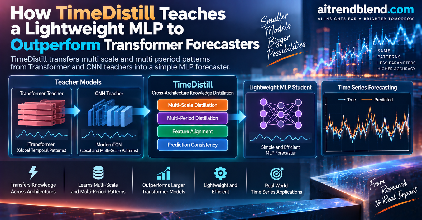
- TimeDistill distills knowledge from Transformer or CNN teacher models into a lightweight MLP for long term time series forecasting.
- Instead of copying raw predictions, it aligns multi scale temporal patterns and multi period frequency patterns between student and teacher.
- The distilled MLP beats standalone MLP performance by as much as 18.6 percent and often beats the teacher itself, on eight widely used benchmarks.
- Inference runs up to seven times faster and the model uses up to one hundred thirty times fewer parameters than the teachers it learns from.
- A theoretical result frames the method as a form of mixup augmentation, blending ground truth with teacher signals rather than simply copying them.
The debate the paper is actually trying to settle
Forecasting research has spent the last few years arguing with itself. Transformers arrived promising to capture long range dependencies across a time series, and models like Informer and Autoformer chased that promise with increasingly elaborate attention mechanisms. Then a 2023 paper from Zeng and colleagues asked a pointed question. Are transformers actually effective for time series forecasting. Their answer, backed by a simple linear model that matched or beat several Transformer baselines, was a fairly blunt no, at least not by default. The field split into two camps after that. One camp kept refining Transformers, producing PatchTST with its patch based tokenization and iTransformer, which inverts the usual axis and treats each variable as a token rather than each timestep. CNN based approaches like ModernTCN pushed convolutional receptive fields wider. The other camp doubled down on simplicity, producing lightweight MLP variants such as TSMixer and LightTS that chase efficiency rather than raw accuracy.
The team behind TimeDistill, Juntong Ni, Zewen Liu, Shiyu Wang, Ming Jin and Wei Jin, noticed that this framing treats the two camps as competitors when they might really be complementary. Their preliminary analysis compared an MLP’s prediction errors against a teacher model’s errors sample by sample, not just averaged across a whole dataset. Averaged across eight benchmarks, the MLP loses to teacher models overall. But when the researchers computed what they call a win ratio, the fraction of individual test windows where the MLP actually beats the teacher, the number came out close to fifty percent on most datasets. On the Traffic dataset specifically, the MLP trails ModernTCN in aggregate yet wins on 81 percent of individual samples. Different architectures are apparently good at different slices of the data, and neither one dominates everywhere.
Why matching predictions directly does not work well
The obvious move at this point is standard knowledge distillation, introduced by Hinton and colleagues back in 2015, where a small student network is trained to mimic a larger teacher’s output distribution rather than just the ground truth labels. Applying that directly to forecasting sounds simple. Train the MLP to match the teacher’s predicted future values alongside the true values. The authors tried a version of this and found three separate problems.
First, a teacher’s raw predictions carry their own noise, and asking a small model to fit that noise exactly can make training less stable than just fitting the ground truth would have been. Second, an MLP with limited capacity struggles to replicate a teacher’s fine grained trend and seasonality behavior from the output values alone, since a single vector of predicted numbers does not expose the structure that produced them. Third, matching only the final predictions throws away everything in the teacher’s intermediate representations, which is often where the richer and more transferable knowledge actually lives. The team needed a way to hand the MLP something more structured than a list of predicted numbers.
What TimeDistill actually distills
The paper’s core move is to stop asking what the teacher predicted and start asking what patterns the teacher’s predictions contain. Two categories of pattern turn out to matter for time series specifically, and the authors build a small preliminary study around each one before proposing their method.
Multi scale patterns in the temporal domain
Real time series rarely live at a single resolution. Hourly traffic counts show sharp daily commuting spikes, but if you average those same counts into daily totals you start to see holiday effects and weekly rhythms instead. A forecasting model that only nails the finest resolution but drifts on the coarser trend will still produce visibly wrong long horizon forecasts. The authors downsample model predictions with a stride two convolution to generate a stack of coarser views, what they call scales zero through three, and then compare each model’s predictions at every scale against the ground truth. Transformer and CNN teachers track the ground truth closely even at the coarsest scale. The plain MLP does not. It captures fine detail reasonably well but loses the plot on the broader trend, which is exactly the kind of failure a control system downstream would notice first.
Multi period patterns in the frequency domain
The second failure mode shows up when you look at predictions through a Fast Fourier Transform instead of a time axis. Weather data tends to carry both a daily cycle and a slower yearly one. Electricity demand often shows weekly and quarterly rhythms layered on top of each other. Converting predictions into a spectrogram exposes which periodicities a model actually captured, and by how much its amplitude at each frequency departs from the ground truth. On the ECL electricity dataset, the paper reports the MLP undershooting the dominant frequency’s amplitude by roughly 150 units, compared with gaps of 18 to 29 for the Transformer and CNN teachers. The MLP is not blind to periodicity entirely, but it consistently underweights the frequencies that matter most.
Put together, these two studies point toward a specific answer to the paper’s central design question. Rather than distilling raw predicted values, TimeDistill distills the multi scale temporal structure and the multi period frequency structure, at both the final prediction level and inside the model’s intermediate feature representations.
How the distillation actually works
The overall setup follows a fairly conventional teacher student split. A teacher network, which can be any Transformer such as iTransformer or PatchTST, or any CNN such as ModernTCN, is pretrained separately and then frozen. Only the student MLP is trained, and it is trained with a combined loss made of the usual supervised forecasting loss plus two additional distillation terms, one for multi scale alignment and one for multi period alignment, each applied at both the prediction level and the feature level.
Multi scale distillation
At the prediction level, both the teacher’s forecast and the student’s forecast are repeatedly downsampled with a temporal stride two convolution, producing a family of predictions at coarser and coarser resolutions. The student is trained to match the teacher’s downsampled predictions at every scale using a mean squared error term.
At the feature level, the same downsampling is applied to the intermediate hidden representations rather than the final outputs. Since the teacher and student feature dimensions rarely match, a small trainable regressor network first projects the teacher’s features into the student’s dimensionality before the multi scale comparison happens. The authors set the number of scales M to three by default, based on a sensitivity sweep that showed diminishing returns beyond that point.
Multi period distillation
For frequency domain alignment, both the teacher’s and the student’s predictions are transformed with an FFT, the direct current component is dropped, and the amplitude spectrum is passed through a softmax with a relatively cold temperature of 0.5. That softmax step matters. It converts a raw amplitude spectrum, which is noisy at less important frequencies, into a sharper probability distribution over which periods actually matter for this window of data.
The student is trained to match this period distribution using KL divergence, again both on the final predictions and, with an added regressor to align dimensions, on intermediate features.
Putting the losses together
The full training objective combines the supervised ground truth loss with the four distillation terms, weighted by two hyperparameters that separately control how much the prediction level and feature level terms contribute.
Crucially, all of this heavy lifting happens during training, while the teacher is frozen and its outputs can even be cached ahead of time. Once training finishes, the teacher is discarded entirely. Only the small MLP ships to production, which is where the reported inference speedups come from.
What the experiments actually show
The team evaluated TimeDistill against eight established forecasting baselines on eight benchmark datasets covering electricity load, four ETT temperature series, solar output, road traffic and weather, using prediction horizons of 96, 192, 336 and 720 steps with a fixed 720 step lookback window. ModernTCN serves as the default teacher, though the paper also reports results using iTransformer, TimeMixer and PatchTST as alternative teachers.
| Dataset | TimeDistill MSE | Best teacher used (ModernTCN) MSE | Standalone MLP MSE |
|---|---|---|---|
| ECL | 0.157 | 0.167 | 0.173 |
| ETTh1 | 0.429 | 0.469 | 0.502 |
| ETTh2 | 0.345 | 0.357 | 0.393 |
| ETTm1 | 0.348 | 0.390 | 0.391 |
| ETTm2 | 0.244 | 0.267 | 0.300 |
| Solar | 0.184 | 0.191 | 0.194 |
| Traffic | 0.387 | 0.413 | 0.434 |
| Weather | 0.220 | 0.238 | 0.234 |
Averaged across all prediction horizons, TimeDistill posts the lowest mean squared error on seven of the eight datasets and the lowest mean absolute error on all eight, edging out iTransformer on ECL and Traffic even though those are not the datasets’ respective default teachers. Relative to the ModernTCN teacher it distills from by default, the improvement reaches 5.37 percent, and relative to a standalone MLP trained without any distillation, the improvement reaches 13.87 percent. The paper also reports gains of up to 21.41 percent over a teacher when using TimeMixer specifically, which suggests the framework is not narrowly tuned to one teacher architecture.
The efficiency side of the results is where the practical case gets made. On the ECL dataset, TimeDistill’s underlying MLP runs inference in about 1.1 milliseconds per batch with roughly 1.1 million parameters, against ModernTCN’s 6.2 milliseconds and 132 million parameters. Compared with the much older Autoformer baseline, the speedup reaches 196 times. The paper frames this as up to seven times faster inference and up to one hundred thirty times fewer parameters than the teacher models it draws from, figures that hold up given the reported per model latency and parameter counts.
What the ablations rule out
Removing either the multi scale loss or the multi period loss individually still leaves TimeDistill ahead of a standalone MLP, which tells you neither component is doing all the work alone. Removing both the feature level terms hurts more than removing the prediction level terms on most datasets, a result the authors read as evidence that a teacher’s intermediate representations carry more transferable signal than its final output values do. Perhaps the most striking ablation drops the supervised ground truth loss entirely, training the MLP purely on distillation signals. Performance still beats both the plain MLP and, in most cases, the teacher itself. The explanation the authors offer is that raw ground truth is noisier and harder to fit directly than the smoothed, teacher informed targets the distillation losses provide, which lines up with the mixup interpretation from the theory section.
Where this framework could go next, and where it might not help
The authors test TimeDistill’s adaptability along three axes. Swapping in TSMixer, LightTS and the extremely lightweight FITS as students instead of a plain MLP still produces consistent gains, between roughly 4 and 8 percent MSE reduction depending on the student, which suggests the method generalizes beyond one specific architecture. Stretching or shrinking the lookback window from 96 to 720 steps, TimeDistill stays ahead of both the teacher and the plain MLP at every length tested. And in a smaller side analysis, the authors visualize inter variable correlation matrices and find that TimeDistill’s student, despite being trained in a channel independent way that never explicitly models relationships between variables, ends up with a correlation structure that resembles the channel dependent teacher’s far more than a plain MLP’s does. That is a genuinely interesting side effect the paper flags as future work rather than something it fully explains.
Honest limitations
The framework’s benefit is not guaranteed everywhere. When a teacher itself performs badly on a dataset, distilling from it can hurt rather than help. The paper’s own appendix shows the Autoformer teacher, which performs particularly poorly on the Solar dataset, dragging the distilled student’s mean absolute error down by 29 percent relative to a plain MLP, a case where the teacher is simply not worth learning from. The hyperparameters that weight the prediction level and feature level losses need dataset specific tuning within a fairly narrow search range, and the paper reports the optimal balance shifts depending on how large the initial gap between the MLP and its teacher already is. The multi period gain is also uneven. On some datasets removing it barely changes results because the teacher’s frequency distribution was already close to the ground truth, so there was little extra signal for that loss term to transfer in the first place. Finally, all of the reported results use a fixed 720 step lookback window and channel independent MLP students, so how well the approach holds up on very short context windows or on datasets with far more extreme non stationarity than these eight benchmarks remains an open question the paper does not directly test.
The broader implication for anyone deploying forecasting models
Step back from the specific architecture choices and TimeDistill is really making a case about how to think about the efficiency versus accuracy tradeoff. The usual instinct when a lightweight model underperforms is to make it bigger, or to accept the accuracy hit as the cost of deployment speed. This paper suggests a third option that sits between those two, using an expensive model purely as a training time teacher and then throwing it away once its knowledge has been distilled into something cheap enough to actually run in production. That pattern is not unique to forecasting. It echoes what BERT distillation did for NLP inference and what pruning based approaches have done for vision models, but time series forecasting has lacked an architecture aware version of it until now. Given how many industrial forecasting pipelines already run lightweight linear or MLP models purely for latency reasons, a training recipe that closes part of the accuracy gap without touching the deployed architecture at all is the kind of result that is easy to adopt without re-engineering an existing pipeline. Whether it becomes a standard step in production forecasting workflows will likely depend on how well it generalizes past the eight academic benchmarks tested here, particularly on the messier, more irregular series that show up in real operational data.
Full PyTorch implementation
The following implementation reconstructs the core TimeDistill training loop described in the paper, including the multi scale downsampling, the multi period FFT and softmax distillation, and the combined loss from Equation 12. It is written to run as a standalone smoke test on synthetic data so you can verify the mechanics before plugging in a real teacher checkpoint and dataset.
# timedistill.py
# Reconstructed implementation of the TimeDistill cross architecture
# distillation framework for long term time series forecasting.
# Reference: Ni, Liu, Wang, Jin and Jin, "TimeDistill: Efficient Long-Term
# Time Series Forecasting with MLP via Cross-Architecture Distillation", KDD 2026.

import torch
import torch.nn as nn
import torch.nn.functional as F


class SeriesDecomposition(nn.Module):
    """Simple moving average trend and residual decomposition,
    used ahead of the student MLP as in the paper's Appendix B."""

    def __init__(self, kernel_size: int = 25):
        super().__init__()
        self.kernel_size = kernel_size
        self.avg = nn.AvgPool1d(kernel_size=kernel_size, stride=1, padding=0)

    def forward(self, x: torch.Tensor):
        # x: (batch, time, channels)
        pad = (self.kernel_size - 1) // 2
        front = x[:, 0:1, :].repeat(1, pad, 1)
        end = x[:, -1:, :].repeat(1, self.kernel_size - 1 - pad, 1)
        padded = torch.cat([front, x, end], dim=1)
        trend = self.avg(padded.permute(0, 2, 1)).permute(0, 2, 1)
        residual = x - trend
        return residual, trend


class StudentMLP(nn.Module):
    """Channel independent MLP student. Each variable is forecast
    independently, matching the paper's default channel independent
    strategy described in Appendix B."""

    def __init__(self, lookback: int, horizon: int, hidden_dim: int = 512):
        super().__init__()
        self.decomp = SeriesDecomposition()
        self.seasonal_proj = nn.Sequential(
            nn.Linear(lookback, hidden_dim),
            nn.GELU(),
            nn.Linear(hidden_dim, horizon),
        )
        self.trend_proj = nn.Linear(lookback, horizon)
        self.feature_head = nn.Linear(lookback, hidden_dim)

    def forward(self, x: torch.Tensor):
        # x: (batch, lookback, channels)
        residual, trend = self.decomp(x)
        residual = residual.permute(0, 2, 1)
        trend = trend.permute(0, 2, 1)
        seasonal_out = self.seasonal_proj(residual)
        trend_out = self.trend_proj(trend)
        prediction = (seasonal_out + trend_out).permute(0, 2, 1)
        # intermediate feature, used for feature level distillation
        feature = self.feature_head(residual)
        return prediction, feature


class FeatureRegressor(nn.Module):
    """Projects teacher features into the student's feature
    dimension before multi scale and multi period feature matching,
    as described around Equation 5 in the paper."""

    def __init__(self, teacher_dim: int, student_dim: int):
        super().__init__()
        self.proj = nn.Sequential(
            nn.Linear(teacher_dim, student_dim),
            nn.GELU(),
            nn.Linear(student_dim, student_dim),
        )

    def forward(self, teacher_feature: torch.Tensor):
        return self.proj(teacher_feature)


def multi_scale_series(x: torch.Tensor, num_scales: int = 3):
    """Equation 3. Downsamples along the time axis with a stride two
    1D convolution, producing scales 0 through num_scales."""
    # x: (batch, time, channels) -> operate per channel
    batch, time, channels = x.shape
    scales = [x]
    current = x.permute(0, 2, 1).reshape(batch * channels, 1, time)
    kernel = torch.ones(1, 1, 2, device=x.device) / 2.0
    for _ in range(num_scales):
        current = F.conv1d(current, kernel, stride=2)
        downsampled = current.reshape(batch, channels, -1).permute(0, 2, 1)
        scales.append(downsampled)
        if current.shape[-1] < 2:
            break
    return scales


def multi_scale_loss(teacher_scales, student_scales):
    """Equation 4 and Equation 6. Averages MSE across every matched
    scale between teacher and student."""
    n = min(len(teacher_scales), len(student_scales))
    total = 0.0
    for m in range(n):
        total = total + F.mse_loss(student_scales[m], teacher_scales[m])
    return total / n


def period_distribution(x: torch.Tensor, temperature: float = 0.5):
    """Equations 7 and 8. FFT amplitude spectrum with the DC
    component removed, softened by a cold temperature softmax."""
    # x: (batch, time, channels)
    spectrum = torch.fft.rfft(x, dim=1)
    amplitude = spectrum.abs()
    amplitude = amplitude[:, 1:, :]  # drop the DC component
    return F.softmax(amplitude / temperature, dim=1)


def multi_period_loss(teacher_pred: torch.Tensor, student_pred: torch.Tensor, temperature: float = 0.5):
    """Equation 9. KL divergence between teacher and student
    period distributions."""
    q_teacher = period_distribution(teacher_pred, temperature)
    q_student = period_distribution(student_pred, temperature)
    log_q_student = torch.log(q_student.clamp_min(1e-8))
    return F.kl_div(log_q_student, q_teacher, reduction="batchmean")


def timedistill_loss(
    ground_truth: torch.Tensor,
    student_pred: torch.Tensor,
    student_feature: torch.Tensor,
    teacher_pred: torch.Tensor,
    teacher_feature_aligned: torch.Tensor,
    alpha: float = 0.5,
    beta: float = 0.5,
    num_scales: int = 3,
    temperature: float = 0.5,
):
    """Equation 12. Combines the supervised loss with prediction level
    and feature level multi scale and multi period distillation."""
    sup_loss = F.mse_loss(student_pred, ground_truth)

    student_scales = multi_scale_series(student_pred, num_scales)
    teacher_scales = multi_scale_series(teacher_pred, num_scales)
    scale_loss_y = multi_scale_loss(teacher_scales, student_scales)

    student_feat_scales = multi_scale_series(student_feature, num_scales)
    teacher_feat_scales = multi_scale_series(teacher_feature_aligned, num_scales)
    scale_loss_h = multi_scale_loss(teacher_feat_scales, student_feat_scales)

    period_loss_y = multi_period_loss(teacher_pred, student_pred, temperature)
    period_loss_h = multi_period_loss(teacher_feature_aligned, student_feature, temperature)

    total = (
        sup_loss
        + alpha * (scale_loss_y + period_loss_y)
        + beta * (scale_loss_h + period_loss_h)
    )
    return total, {
        "sup": sup_loss.item(),
        "scale_y": scale_loss_y.item(),
        "period_y": period_loss_y.item(),
        "scale_h": scale_loss_h.item(),
        "period_h": period_loss_h.item(),
    }


def train_step(student, regressor, teacher, optimizer, x, y, alpha=0.5, beta=0.5):
    """One training step. The teacher stays frozen throughout, as
    specified in Section 4.3 of the paper."""
    student.train()
    optimizer.zero_grad()

    student_pred, student_feature = student(x)

    with torch.no_grad():
        teacher_pred, teacher_feature_raw = teacher(x)
    teacher_feature_aligned = regressor(teacher_feature_raw)

    loss, parts = timedistill_loss(
        ground_truth=y,
        student_pred=student_pred,
        student_feature=student_feature,
        teacher_pred=teacher_pred,
        teacher_feature_aligned=teacher_feature_aligned,
        alpha=alpha,
        beta=beta,
    )
    loss.backward()
    optimizer.step()
    return loss.item(), parts


@torch.no_grad()
def evaluate(student, data_loader):
    """Computes MSE and MAE across a validation or test loader,
    matching Equations 15 and 16 in Appendix B."""
    student.eval()
    total_mse, total_mae, count = 0.0, 0.0, 0
    for x, y in data_loader:
        pred, _ = student(x)
        total_mse += F.mse_loss(pred, y, reduction="sum").item()
        total_mae += F.l1_loss(pred, y, reduction="sum").item()
        count += y.numel()
    return total_mse / count, total_mae / count


class DummyTeacher(nn.Module):
    """Stand in teacher for the smoke test below. In practice this
    would be a frozen, pretrained iTransformer, PatchTST or ModernTCN."""

    def __init__(self, lookback: int, horizon: int, feature_dim: int = 128):
        super().__init__()
        self.proj = nn.Linear(lookback, horizon)
        self.feature_head = nn.Linear(lookback, feature_dim)

    def forward(self, x: torch.Tensor):
        x_t = x.permute(0, 2, 1)
        pred = self.proj(x_t).permute(0, 2, 1)
        feature = self.feature_head(x_t)
        return pred, feature


def smoke_test():
    """Runs one forward and backward pass on random dummy data to
    confirm every shape and loss term is wired correctly."""
    torch.manual_seed(0)
    batch, lookback, horizon, channels = 8, 96, 96, 7

    x = torch.randn(batch, lookback, channels)
    y = torch.randn(batch, horizon, channels)

    student = StudentMLP(lookback=lookback, horizon=horizon, hidden_dim=128)
    teacher = DummyTeacher(lookback=lookback, horizon=horizon, feature_dim=128)
    for p in teacher.parameters():
        p.requires_grad_(False)

    regressor = FeatureRegressor(teacher_dim=128, student_dim=128)
    optimizer = torch.optim.Adam(
        list(student.parameters()) + list(regressor.parameters()), lr=1e-2
    )

    loss, parts = train_step(student, regressor, teacher, optimizer, x, y)
    print(f"total loss {loss:.4f}")
    for name, value in parts.items():
        print(f"  {name}: {value:.4f}")

    assert torch.isfinite(torch.tensor(loss)), "loss is not finite"
    print("smoke test passed")


if __name__ == "__main__":
    smoke_test()
Conclusion
What TimeDistill demonstrates, once you strip away the specific loss functions, is that the accuracy gap between lightweight and heavyweight forecasting models is not entirely a capacity problem. Part of it is a training signal problem. The plain MLP in these experiments already had a fifty percent win ratio against its teacher before any distillation happened, which means the raw representational capacity to compete was sitting there unused. What was missing was a way to point that capacity at the specific structures, coarse trends and dominant periodicities, that the model was failing to learn from ground truth labels alone.
The conceptual shift is subtle but important. Most distillation work in vision and language treats the teacher’s output distribution as the thing worth copying. TimeDistill instead treats the teacher as a source of two very specific, domain appropriate signals, and it is precisely that domain awareness, choosing multi scale and multi period structure rather than generic feature matching, that produces the gains reported here. The theoretical framing as a mixup variant reinforces why this works rather than just showing that it does, since a softened, blended target is a well understood way to fight overfitting and noise sensitivity in a small model.
Transferability beyond forecasting seems plausible but unproven in this paper. The authors gesture toward foundation model teachers and multivariate extensions as future work rather than testing them here, and the short term forecasting results on the PEMS traffic datasets in the appendix are described as preliminary rather than a core contribution. Anyone hoping to apply the same multi scale and multi period framing to a different sequence modeling task, audio or sensor data for instance, would be extrapolating past what the paper actually validates.
The honest remaining limitations matter more than they might first appear. A distillation framework is only as good as its teacher, and the Solar dataset result with Autoformer as teacher is a clear demonstration that a poorly performing teacher can actively hurt the student rather than help it. Practitioners adopting this approach would need to validate their chosen teacher’s quality before trusting the distillation process to compensate for its weaknesses, and the dataset specific hyperparameter tuning the paper describes suggests this is not yet a fully turnkey recipe.
Even with those caveats, the practical case here is hard to dismiss. A model that costs almost nothing to run, achieved through a training time procedure that never touches the production architecture at all, is exactly the kind of result that tends to get adopted quietly and quickly once teams notice it exists. The bigger story is less about time series specifically and more about a general principle worth remembering the next time a small model seems stuck underperforming a large one. Sometimes the fix is not a bigger model. It is better information about what the model should be paying attention to.
Frequently asked questions
What is TimeDistill in simple terms
TimeDistill is a training method that helps a small, fast MLP model learn to forecast time series almost as well as a much larger Transformer or CNN model, by having the MLP copy specific temporal and frequency patterns from the larger model during training rather than copying its raw predictions.
Does the final deployed model still need the teacher network
No. The teacher is only used during training and is discarded afterward. The deployed model is the small MLP by itself, which is why the reported inference speed and parameter count improvements hold at deployment time.
Which teacher models does TimeDistill work with
The paper tests iTransformer, ModernTCN, TimeMixer and PatchTST as teachers, and reports smaller scale results with additional teachers including MICN, FEDformer, TimesNet and Autoformer in its appendix. The framework is not tied to one specific teacher architecture.
How much faster is the distilled MLP than the teacher models
On the ECL electricity dataset, the paper reports up to seven times faster inference and up to one hundred thirty times fewer parameters compared with the teacher models tested, with a 196 times speedup reported specifically against the older Autoformer baseline.
Can TimeDistill make a bad forecasting model good
Not reliably. The paper’s own results show that distilling from a poorly performing teacher, such as Autoformer on the Solar dataset, can make the student worse rather than better. The teacher’s quality still sets an upper bound on how much the method can help.
Is the code for TimeDistill publicly available
The paper states that code is available through a linked GitHub repository referenced in the abstract. Readers should check the paper itself, linked below, for the current repository address.
Read the original research
This analysis covers the key ideas from the paper. For the full experimental tables, proofs and appendix material, read the source directly.
Related reading
Ni, J., Liu, Z., Wang, S., Jin, M. and Jin, W. TimeDistill. Efficient Long Term Time Series Forecasting with MLP via Cross Architecture Distillation. Proceedings of the 32nd ACM SIGKDD Conference on Knowledge Discovery and Data Mining, KDD 2026. arXiv:2502.15016.
This analysis is based on the published paper and an independent evaluation of its claims.
Pingback: U-Mamba2-SSL: The Groundbreaking AI Framework Revolutionizing Tooth & Pulp Segmentation in CBCT Scans - aitrendblend.com
Pingback: Stabilizing Uncertain Stochastic Systems: A Deep Learning Approach to Inverse Optimal Control - aitrendblend.com
Pingback: Revolutionary AI Breakthrough: How Anatomy-Guided Deep Learning Is Transforming Breast Cancer Detection in PET-CT Scans - aitrendblend.com
Your article helped me a lot, is there any more related content? Thanks! https://accounts.binance.com/register-person?ref=IHJUI7TF