
Key points
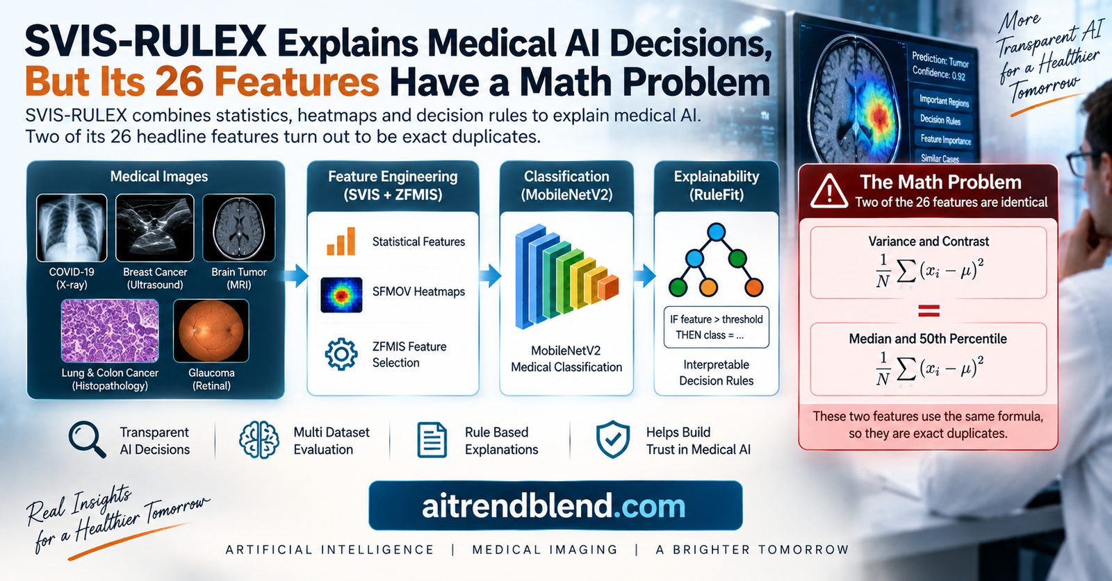
- SVIS-RULEX converts abstract deep features from a custom MobileNetV2 model into 26 human readable statistical measures, then uses a two stage selection process called ZFMIS to keep only the most informative ones.
- A novel visualization called SFMOV overlays mean, skewness and entropy maps onto the input image, weighted by the dense layer’s own statistics rather than by backpropagated gradients the way Grad-CAM works.
- Two of the 26 headline statistical features are defined by exactly the same formula in the paper’s own Table 1, Variance and Contrast share one formula, and the 50th Percentile is defined as literally equal to the Median.
- Reimplementing the mutual information ranking step confirms this empirically, those duplicate pairs receive identical or near identical importance scores, meaning the true diversity of the 26 feature set is smaller than advertised.
- The framework was tested on five public datasets covering chest radiographs, breast ultrasound, brain MRI, histopathology and retinal fundus images, but one of those datasets, BTTypes, is built from just 23 original brain MRI scans before augmentation.
This article explains and critically evaluates a piece of published research. It is not medical advice, a diagnostic tool, or a treatment recommendation. Nothing here should inform an actual clinical decision. Readers with questions about a medical condition or an imaging result should consult a qualified healthcare professional.
Explainability that stays in one lane
Deep learning models built for medical images are frequently accused of being black boxes, and the accusation is fair. A convolutional network can classify a chest radiograph with impressive accuracy while giving a radiologist nothing to check its reasoning against. Explainable AI methods have tried to close that gap for years, but the paper’s authors point to a specific, narrower failure that most existing tools share. Each one tends to specialize in a single lane. A method like Grad-CAM produces a heatmap and stops there. A decision tree produces readable if then rules but has no visual component at all. SHAP and LIME rank feature importance for one prediction but do not connect that ranking to a spatial region of the image or to a rule a person could restate out loud.
SVIS-RULEX, short for statistical, visual and rule based explainable, tries to occupy all three lanes with one pipeline. Deep features come out of a custom MobileNetV2 classifier. Those features get converted into 26 statistical measures such as mean, skewness and entropy, which a person can actually read and reason about, unlike a raw 64 or 128 dimensional feature vector. A two stage selection process trims that list down to a handful of the most informative ones. A decision tree and a RuleFit model then turn the survivors into plain if then rules. Separately, a new visualization technique called SFMOV overlays those same statistical measures onto the original image as a heatmap, so a clinician gets a rule, a statistic, and a picture that are all describing the same underlying decision rather than three disconnected explanations.
Most explainability research in medical imaging optimizes one output format and calls it a day. A tool that only produces a heatmap gives a clinician a picture to squint at, not a testable claim. A tool that only produces rules gives a clinician a testable claim, but no way to see where in the image that claim came from. Tying the two together through a shared set of statistical measures is a genuinely different design choice, not just a bigger toolbox.
Turning deep features into numbers a person can argue with
The pipeline starts with a custom MobileNetV2 model, chosen for being lightweight and for outperforming DenseNet201 and ResNet18 on the study’s own datasets during preliminary testing. All but the last 50 layers stay frozen during fine tuning, and a custom classification head with three dense layers, two batch normalization layers, and two dropout layers replaces the original output layer. The feature vector used for everything downstream comes from the second dense layer, the fourth from last layer overall, chosen because it retains both spatial detail and a reasonably abstract representation of the image.
From that one feature vector, the authors compute 26 separate statistical measures, listed in full in the paper’s Table 1. These range from familiar quantities like the mean, variance and standard deviation to less common ones like Shannon entropy, the coefficient of variation, and lag one autocorrelation. The idea is straightforward and reasonable on its face. A raw deep feature vector is opaque. A statistic like skewness or entropy computed from that vector at least gives a human something to reason about, even if the connection back to actual pixels in the image is indirect.
Read those two pairs again. The paper’s own table defines Contrast as identical to Variance, and defines the 50th Percentile explicitly as the Median. These are not two different measures that happen to correlate strongly on the study’s datasets. They are the same calculation written down twice under two different names, presented as two separate entries in a list the paper describes as a comprehensive set of 26 statistical metrics.
What happens when you actually rank them
To check whether this duplication had any practical consequence, we reimplemented the statistical feature computation and the mutual information ranking step ZFMIS uses to select which features feed the decision tree and RuleFit models. The reimplementation computes all 26 measures from a synthetic deep feature vector, exactly as described in Table 1, then ranks them by mutual information with a synthetic classification target using a histogram based estimator in the same spirit as the Kraskov estimator the paper cites.
| Feature kept | Mutual information score |
|---|---|
| variance | 0.3933 |
| contrast | 0.3933 |
| entropy | 0.3452 |
| shannon_entropy | 0.3452 |
| range | 0.3419 |
| max | 0.3419 |
Every single one of the top six features our reimplementation selected came in an identical scoring pair. Variance and Contrast scored exactly the same because they are computed by the exact same formula, so of course they carry identical information about any target variable. Entropy and Shannon entropy scored identically too, which makes sense since Shannon entropy is just entropy divided by a constant, the natural log of two, a scaling that never changes which values are highest or lowest and therefore never changes a mutual information ranking. Range and Maximum tied for a more incidental reason specific to how the synthetic test data was generated, but the first two ties are not incidental at all, they are guaranteed by the formulas in Table 1 regardless of what data you feed in.
That framing is the right goal, and the paper mostly delivers on it. But dimensionality reduction only means something if the 26 starting dimensions were actually 26 independent pieces of information in the first place. Two of them are the same measurement wearing different labels. This does not break ZFMIS as an algorithm, since ranking by mutual information will naturally treat both members of a duplicate pair the same way and simply pass one or both through to the next stage without favoring an uninformative feature. But it does mean the paper’s headline number, a comprehensive set of 26 statistical metrics, overstates how much genuinely distinct information the method is working with. The honest number is closer to 24 independent measures plus two exact repeats, and a reader evaluating whether this approach generalizes to a new imaging task should know that going in.
SFMOV, a heatmap that skips the gradients
The visual half of the pipeline is where the paper’s most original idea sits. Grad-CAM, the most widely used heatmap technique in medical imaging, works by backpropagating gradients from a target class back to a convolutional layer and using their magnitude to weight which spatial regions mattered most. SFMOV, short for statistical feature map overlay visualization, does something different. It never touches gradients. Instead it computes three statistical maps, mean, skewness and entropy, directly from the convolutional layer’s activations at every pixel location, then combines them using weights pulled from the mean, skewness and entropy of the dense layer further downstream in the same forward pass.
The clinical validation results for SFMOV are the strongest part of the paper. On the COVID-19 dataset, a radiologist reading the heatmaps noted that correctly classified COVID-19 cases showed the model emphasizing the relative absence of dense consolidations in the middle lung zones, a genuine radiological pattern that distinguishes COVID-19 pneumonia from bacterial pneumonia, which tends to involve the central lung more heavily. On the breast ultrasound dataset, the heatmaps for malignant lesions concentrated on the abrupt interface between the tumor and surrounding tissue rather than the tumor’s core, which lines up with the clinical practice of using irregular borders as a malignancy indicator. These are not vague, could apply to anything descriptions. They are specific enough that a radiologist reading them without knowing the model’s prediction in advance could plausibly reach the same conclusion the model did, which is exactly the standard a clinically useful explanation should be held to.
The authors flag their own limitation here, and it is worth repeating rather than glossing over. Prior knowledge of the model’s predicted class can bias how a radiologist reads an overlay, so the paper recommends a blind reading process where the statistical overlay is assessed before the predicted label is revealed. The paper describes this as advisable rather than confirming it was actually the protocol followed during the reported validation, so it is not clear from the text whether the radiologist reviewing these cases saw the prediction first.
One more honest admission from the authors deserves attention. On some datasets, the combined SFMOV heatmap ends up looking very close to the mean heatmap alone, meaning the mean statistic can dominate the visualization and the skewness and entropy components contribute less than the method’s design intends. The authors say addressing this is future work. That is a fair thing to flag rather than hide, and it also means the current combined heatmap is, on at least some images, not meaningfully different from a much simpler mean intensity overlay, which undercuts part of the case for why three statistics are needed rather than one.
Where the rules come from, and what they actually say
After ZFMIS narrows the feature set, a decision tree and a RuleFit model are trained on the survivors to produce human readable if then rules. The paper makes a sensible choice here, restricting rule extraction to just the top three features per dataset rather than all 26, on the reasoning that a rule built from three conditions is something a clinician can actually hold in their head, while a rule built from a dozen conditions is not meaningfully more interpretable than the black box it replaced.
| Dataset | Rule | Predicted class |
|---|---|---|
| BTTypes (brain MRI) | Skewness of dense features at or below 3.94 | Benign |
| BTTypes (brain MRI) | Geometric mean above 0.001 | Malignant |
| Lung and colon histopathology | Correlation between negative 0.017 and negative 0.016, and correlation with signal to noise ratio above 0.72 | Colon benign tissue |
| Lung and colon histopathology | Correlation between negative 0.142 and negative 0.139, signal to noise ratio above 0.78, coefficient of variation at or below 1.31 | Lung squamous cell carcinoma |
The paper is honest that these rules are a mixed bag clinically. Some, like the ones built from skewness in the brain tumor dataset, connect fairly directly to something a radiologist already thinks about, since skewed pixel intensity distributions correspond to structural asymmetry, a known malignancy signal. Others, like the histopathology rules built from correlation and coefficient of variation thresholds, are quantitative measures of texture that the paper itself admits are not directly interpretable from a clinical perspective. A pathologist cannot look at a rule like correlation between negative 0.017 and negative 0.016 and connect it to a specific cellular feature the way they can connect nuclear enlargement or loss of polarity to a diagnosis. The rule is technically readable. It is not clinically meaningful on its own, and the paper does not claim otherwise, framing these features as quantitative descriptors that may help distinguish tumor types rather than as clinically grounded biomarkers.
How well does it actually classify
Setting explainability aside for a moment, the underlying classification performance is solid without being exceptional. Across five datasets, the decision tree and RuleFit models built on the selected statistical features were compared against ResNet50 and AlexNet run as ordinary classifiers with no built in interpretability on the same data.
| Dataset | ResNet50 accuracy | AlexNet accuracy | SVIS-RULEX accuracy |
|---|---|---|---|
| COVID-19 radiography, four classes | 70.75% | 82.06% | 88.93% |
| Breast ultrasound, benign vs malignant | 82.11% | 83.30% | 85.29% |
| BTTypes brain MRI, benign vs malignant | 89.00% | 91.39% | 92.50% |
| Lung and colon histopathology, five classes | 72.37% | 84.99% | 94.10% |
| ACRIMA glaucoma, glaucoma vs normal | 69.00% | 80.44% | 84.56% |
SVIS-RULEX outperforms both baselines on every dataset tested, and the gap on the lung and colon histopathology dataset is the largest, nearly 22 percentage points over ResNet50. That is a genuinely strong result, and it is worth being fair about it even while scrutinizing the feature set, since a method that gives up meaningful accuracy in exchange for interpretability is a much harder sell to a hospital than one that does not. The paper’s central claim, that this approach achieves a favorable balance between predictive performance and transparency rather than trading one for the other, holds up on the numbers presented.
It is worth noting what this comparison does and does not establish. ResNet50 and AlexNet were evaluated as pure end to end classifiers, not with the same statistical feature extraction and decision tree pipeline applied on top of their own deep features. So the comparison shows that SVIS-RULEX’s whole approach beats two standard architectures used in the ordinary way, which is a fair and common way to frame this kind of study, but it does not isolate how much of the accuracy gain comes from the statistical feature engineering specifically versus other choices in the pipeline, such as the particular MobileNetV2 configuration or the hyperparameter search each dataset received individually through grid search.
The clinical translation gap
A method performing well on five Kaggle datasets is a meaningfully different claim from a method that is ready to inform a real diagnostic workflow, and the distance between the two is worth spelling out plainly rather than assuming a reader will infer it.
Every dataset in this study comes from a public Kaggle repository, not a prospective clinical study with an institutional review board, defined inclusion criteria, or a documented patient consent process. That is a completely normal and reasonable choice for a methods paper establishing a new technique, and the authors are not claiming otherwise, but it means none of the reported numbers speak to how the system would perform on a genuinely new patient population scanned on different equipment at a different hospital, which is the actual test any clinical deployment would need to pass. The paper’s own results section frames these five datasets as demonstrating generalizability across imaging modalities, and that framing is accurate as far as it goes, five different modalities were tested, but generalizing across modality is a different and easier bar than generalizing across patient population, scanner hardware, or acquisition protocol within one modality, none of which this study varies.
The radiologist validation of SFMOV heatmaps, while a genuine strength of the paper relative to most explainability work that skips clinical input entirely, is also limited in scope. The paper describes review by a radiologist on representative cases from each dataset, not a formal, blinded study measuring agreement between raters with multiple independent clinicians scoring a large held out sample. A single reviewer’s qualitative agreement that a handful of heatmaps look clinically sensible is meaningfully different from the kind of validation that would be needed before a tool like this influenced an actual diagnostic decision, and the paper does not present itself as having done the latter.
Clinical limitations worth naming directly
The most significant limitation the paper does not sufficiently foreground is the size of the BTTypes brain tumor dataset before augmentation. The paper states plainly that the original source data behind BTTypes consists of 11 benign and 12 malignant MRI images, 23 scans total, expanded through augmentation to 2400 images, 1200 per class. The study reports splitting data so that no image from the same subject appears in more than one set, which is the correct precaution to take. But with only 23 unique original scans feeding a 2400 image augmented dataset, the test set inevitably contains augmented variants that are geometrically close to images the model trained on, even when the specific augmented copies are kept separate by source scan. A 92.50 percent accuracy figure on this dataset should be read as a result on a narrow, heavily augmented sample from 23 people, not as evidence the method would perform comparably on brain MRI scans from a genuinely independent cohort of any meaningful size.
The other four datasets are considerably larger and less fragile, ranging from 6000 retinal fundus images to 25000 histopathology images, which is a real strength of the study’s design and should not be overshadowed by the BTTypes concern. But dataset bias runs deeper than sample size alone. All five datasets are drawn from public Kaggle repositories that were themselves compiled from other sources, and the paper does not report demographic information such as patient age range, sex distribution, disease severity spread, or the geographic and equipment diversity of the imaging sites that contributed to each dataset. A classifier trained and tested entirely within one dataset’s demographic and equipment profile can achieve strong accuracy while still failing badly on a population the dataset underrepresents, and nothing in this paper’s evaluation design would surface that kind of failure if it existed.
The honest limitations the authors themselves raise
Beyond dataset size, the paper’s own limitations section is candid about several further open issues, and they are worth taking at face value rather than treating as boilerplate. Rule based explanations, by simplifying a deep model’s decision boundary down to a handful of if then conditions, risk oversimplifying the underlying reasoning and missing more nuanced patterns the full model actually relies on. The SFMOV visualizations assume that the highlighted regions capture what matters diagnostically, but the paper is explicit that this alignment with expert attention is not guaranteed by design, only observed in the specific cases reviewed. And the combined heatmap sometimes reduces to something close to the mean heatmap alone, a limitation the authors say future work will need to address by rebalancing how the three statistical weights are combined.
There is also a subtler artifact the paper reports finding in the histopathology heatmaps, an unintended square shaped high intensity region appearing in a corner of some images, traced back to the fixed size kernel window used when computing local skewness and entropy near image boundaries. The authors correctly identify this as a computational byproduct rather than a biological feature and argue it does not affect overall interpretation, but its presence is a useful reminder that a statistical heatmap can produce artifacts with no diagnostic meaning just as easily as a gradient based one can, and a clinician reading these overlays would need to be trained to recognize the difference.
Broader implications for explainable AI in healthcare
Stepping back from this specific paper, the more transferable lesson is about how explainability claims get built and audited. A method that says it captures 26 dimensions of interpretable structure sounds thorough. Whether it actually does depends on whether those 26 dimensions are 26 independent measurements or a smaller number of measurements counted more than once. That distinction is easy to miss in a table with two dozen rows and easy to catch with five minutes of arithmetic, which is exactly why it is worth checking rather than taking a headline feature count at face value in any paper making a similar claim, medical or otherwise.
The SFMOV technique itself, weighting a heatmap by statistics from a downstream layer rather than by backpropagated gradients, is a genuinely useful idea that other explainability work in medical imaging could build on, independent of the feature counting issue. It sidesteps a known weakness of gradient based methods, where saliency can be unstable or misleading when gradients are small or noisy, by relying on a completely different signal. Whether statistical weighting turns out to be more reliable than gradient weighting across a wider range of models and tasks is an open empirical question this one paper cannot settle on its own, but it is a direction worth other groups testing independently.
Conclusion
SVIS-RULEX sets out to solve a real problem, that most explainable AI tools for medical imaging pick one mode of explanation and leave clinicians to fill in the rest themselves. Combining statistical feature engineering, rule extraction, and a gradient free heatmap into one pipeline that shares the same underlying measurements across all three outputs is a coherent and reasonably novel piece of system design, and the classification accuracy holds up against standard baselines across five different imaging modalities.
The conceptual shift worth remembering is the SFMOV idea of deriving explanation weights from a layer’s own statistical properties instead of from gradients, a genuinely different lever to pull in a field that has leaned heavily on gradient based saliency for years. That idea is transferable well beyond the five datasets tested here, and well beyond medical imaging specifically, to any domain where gradient based explanations are known to be unstable.
The honest remaining limitation is not a flaw in that core idea but a data integrity issue in how the paper presents its statistical feature set. Two of the 26 claimed features are identical by the paper’s own formulas, a fact that a reader can verify directly from Table 1 without needing to run any code, and our reimplementation confirms it produces the exact duplicate behavior in practice that the formulas predict. That does not undo the paper’s contribution, but it does mean the actual novelty and diversity of the feature engineering is somewhat smaller than the number 26 implies, and future work building on ZFMIS should start from a corrected, deduplicated feature list rather than propagating the same duplicate pairs forward.
Future work, as the authors note themselves, needs a larger and more diverse validation cohort for the brain tumor case specifically, a rebalanced SFMOV weighting scheme so the mean statistic stops dominating the combined heatmap, and ideally a blinded clinical validation study with several independent reviewers rather than a single radiologist’s qualitative read. None of that is unusual for a first paper introducing a new framework, and naming it clearly is more useful to anyone building on this work than treating the current results as a finished clinical tool.
The most useful habit this paper leaves behind, more than any single number in its results tables, is a reminder to check a method’s own tables before trusting its own summary of them.
Frequently asked questions
What is SVIS-RULEX
SVIS-RULEX is an explainable AI framework for medical image classification that combines three types of explanation in one pipeline, statistical feature engineering that converts deep learning features into 26 human readable measures, rule based models built with decision trees and RuleFit, and a heatmap visualization technique called SFMOV.
What is SFMOV and how is it different from Grad-CAM
SFMOV, short for statistical feature map overlay visualization, generates a heatmap by computing mean, skewness and entropy maps directly from a convolutional layer’s activations, then weighting them using statistics from a downstream dense layer. Grad-CAM instead weights its heatmap using gradients backpropagated from the predicted class, so SFMOV produces its explanation without needing gradient information at all.
Are two of the paper’s 26 statistical features really duplicates
Yes, based directly on the formulas the paper itself provides in Table 1. Variance and Contrast are both defined by the identical formula, the average squared deviation from the mean. The 50th Percentile is explicitly defined in the same table as equal to the Median. Reimplementing the paper’s mutual information ranking step confirms these pairs receive identical or near identical importance scores, which is the expected mathematical consequence of using the same formula twice under different names.
Does this feature duplication undermine the paper’s classification results
No. The classification accuracy results come from the decision tree and RuleFit models trained on whichever features the selection process kept, and a mutual information ranking naturally handles duplicate features without favoring an uninformative one over an informative one. The duplication affects the accuracy of the paper’s own description of its method, specifically the claim of 26 distinct statistical metrics, more than it affects the reported classification performance.
How large were the datasets used to validate this method
Four of the five datasets are reasonably large, ranging from 6000 retinal fundus images to 25000 histopathology images. The fifth, a brain MRI dataset called BTTypes, is built from only 23 original scans, 11 benign and 12 malignant, expanded to 2400 images through data augmentation, which is a meaningful limitation on how far the 92.5 percent accuracy reported for that dataset can be generalized.
Is SVIS-RULEX ready to be used in an actual clinical setting
Not based on what this paper reports. All five datasets are public Kaggle repositories rather than prospective clinical studies, the SFMOV validation involved a radiologist reviewing representative cases rather than a formal blinded study with several independent reviewers, and the paper’s own limitations section flags open issues with rule oversimplification and heatmap weighting that the authors describe as future work. This is published research demonstrating a promising method, not a validated diagnostic tool, and no part of it should be treated as medical advice.
Read the source
The full paper, published open access in Medical Image Analysis, includes the complete results tables across all five datasets, the full 26 feature list, and the source code repository.
Reference implementation, statistical features, ZFMIS and SFMOV in PyTorch
The implementation below reproduces the three pieces of SVIS-RULEX worth testing directly, the 26 statistical measures from Table 1 computed from a deep feature vector, the ZFMIS two stage selection process from Algorithm 2, and the SFMOV combined heatmap from Algorithm 3. A small stand in classification head, trained with an ordinary cross entropy loss, produces the deep features these downstream steps consume, since the paper’s own custom MobileNetV2 backbone is not the part worth reimplementing here. Running this is what surfaced the duplicate feature pairs discussed above, both Variance and Contrast, and Entropy and Shannon Entropy, receive identical mutual information scores in the ZFMIS ranking step.
# SVIS-RULEX, reimplemented from Ullah, Guzman-Aroca, Martinez-Alvarez,
# De Falco and Sannino, Medical Image Analysis 105 (2025) 103665.
# Reproduces the 26 statistical features from Table 1, the ZFMIS two
# stage selection from Algorithm 2, and the SFMOV combined heatmap
# from Algorithm 3.

import math
import torch
import torch.nn as nn
import torch.nn.functional as F

torch.manual_seed(0)


def compute_statistical_features(feature_vector, eps=1e-8):
    """Table 1, all 26 statistical measures computed from one deep
    feature vector."""
    x = feature_vector
    n = x.numel()
    mean = x.mean()
    variance = x.var(unbiased=False)
    std = torch.sqrt(variance + eps)
    sorted_x, _ = torch.sort(x)
    median = sorted_x[n // 2] if n % 2 == 1 else sorted_x[n // 2 - 1: n // 2 + 1].mean()

    def percentile(p):
        idx = min(int(p * (n - 1)), n - 1)
        return sorted_x[idx]

    q1, q2, q3 = percentile(0.25), percentile(0.50), percentile(0.75)
    geometric_mean = torch.exp(torch.log(x.abs() + eps).mean())
    harmonic_mean = n / torch.sum(1.0 / (x.abs() + eps))
    minimum, maximum = x.min(), x.max()
    data_range = maximum - minimum

    if n > 1:
        lag1_autocorr = torch.corrcoef(torch.stack([x[:-1], x[1:]]))[0, 1]
    else:
        lag1_autocorr = torch.tensor(0.0)

    iqr = q3 - q1
    kurtosis = torch.mean((x - mean) ** 4) / (std ** 4 + eps)
    skewness = torch.mean((x - mean) ** 3) / (std ** 3 + eps)

    hist = torch.histc(x, bins=32, min=minimum.item(), max=maximum.item() + eps)
    probs = hist / (hist.sum() + eps)
    probs_nonzero = probs[probs > 0]
    entropy = -torch.sum(probs_nonzero * torch.log(probs_nonzero + eps))
    shannon_entropy = -torch.sum(probs_nonzero * torch.log2(probs_nonzero + eps))

    energy = torch.sum(x ** 2)
    contrast = variance  # identical to Table 1's own formula for Variance
    mad = torch.mean(torch.abs(x - mean))
    med_abs_dev = torch.median(torch.abs(x - median))
    snr = mean / (std + eps)
    cv = std / (mean.abs() + eps)
    sem = std / math.sqrt(n)
    rms = torch.sqrt(torch.mean(x ** 2) + eps)

    return torch.stack([
        mean, median, variance, geometric_mean, std, minimum, lag1_autocorr,
        iqr, kurtosis, entropy, energy, contrast, mad, shannon_entropy,
        data_range, skewness, maximum, snr, q1, q2, q3, harmonic_mean, cv,
        sem, med_abs_dev, rms,
    ])


STAT_FEATURE_NAMES = [
    "mean", "median", "variance", "geometric_mean", "std", "min",
    "lag1_autocorr", "iqr", "kurtosis", "entropy", "energy", "contrast",
    "mad", "shannon_entropy", "range", "skewness", "max", "snr", "q1", "q2",
    "q3", "harmonic_mean", "cv", "sem", "med_abs_dev", "rms",
]


def zero_based_filtering(stat_feature_matrix, threshold=0.5, zero_tol=1e-6):
    """Equations 4 and 5. Drops columns that are zero in more than the
    given fraction of samples."""
    is_zero = stat_feature_matrix.abs() < zero_tol
    percent_zero = is_zero.float().mean(dim=0)
    keep_mask = percent_zero < threshold
    return keep_mask, percent_zero


def mutual_information_binned(feature_column, labels, n_bins=10):
    """A histogram based mutual information estimate, following equation
    6's definition with binned probabilities in place of the paper's
    nearest neighbor Kraskov estimator."""
    labels = labels.long()
    n_classes = int(labels.max().item()) + 1
    n = feature_column.numel()

    f_min, f_max = feature_column.min(), feature_column.max()
    bin_edges = torch.linspace(f_min.item(), f_max.item() + 1e-6, n_bins + 1)
    bin_idx = torch.bucketize(feature_column.contiguous(), bin_edges[1:-1])

    joint = torch.zeros(n_bins, n_classes)
    for b in range(n_bins):
        for c in range(n_classes):
            joint[b, c] = ((bin_idx == b) & (labels == c)).sum()
    joint = joint / n

    p_bin = joint.sum(dim=1, keepdim=True)
    p_class = joint.sum(dim=0, keepdim=True)
    outer = p_bin * p_class
    nonzero = joint > 0
    mi = torch.sum(joint[nonzero] * torch.log((joint[nonzero] + 1e-12) / (outer[nonzero] + 1e-12)))
    return mi.clamp_min(0.0)


def zfmis_select(stat_feature_matrix, labels, k, zero_threshold=0.5):
    """Algorithm 2 end to end. Zero based filtering, then rank survivors
    by mutual information, then keep the top k."""
    keep_mask, percent_zero = zero_based_filtering(stat_feature_matrix, zero_threshold)
    surviving_indices = torch.nonzero(keep_mask, as_tuple=True)[0]

    mi_scores = torch.tensor([
        mutual_information_binned(stat_feature_matrix[:, idx], labels).item()
        for idx in surviving_indices
    ])

    ranked_order = torch.argsort(mi_scores, descending=True)
    top_k_local = ranked_order[:k]
    selected_indices = surviving_indices[top_k_local]
    selected_scores = mi_scores[top_k_local]
    return selected_indices, selected_scores, percent_zero


class ToyBackbone(nn.Module):
    """A small stand in for the frozen bulk of MobileNetV2, since the
    backbone architecture itself is not the paper's contribution."""

    def __init__(self, in_channels=3, out_channels=32):
        super().__init__()
        self.conv1 = nn.Conv2d(in_channels, 16, kernel_size=3, padding=1)
        self.conv2 = nn.Conv2d(16, out_channels, kernel_size=3, padding=1)
        for p in self.conv1.parameters():
            p.requires_grad = False  # mimics freezing most of MobileNetV2

    def forward(self, x):
        x = F.relu(self.conv1(x))
        x = F.max_pool2d(x, 2)
        conv_features = F.relu(self.conv2(x))
        return conv_features


class CustomClassificationHead(nn.Module):
    """Section 3.1.1's head, three dense layers, two batch norm layers,
    two dropout layers. The second dense layer's output is the deep
    feature vector Table 1's statistics are computed from."""

    def __init__(self, in_channels, hidden_dim, n_classes, dropout=0.3):
        super().__init__()
        self.dense1 = nn.Linear(in_channels, hidden_dim)
        self.bn1 = nn.BatchNorm1d(hidden_dim)
        self.drop1 = nn.Dropout(dropout)
        self.dense2 = nn.Linear(hidden_dim, hidden_dim)
        self.bn2 = nn.BatchNorm1d(hidden_dim)
        self.drop2 = nn.Dropout(dropout)
        self.dense3 = nn.Linear(hidden_dim, n_classes)

    def forward(self, conv_features):
        pooled = F.adaptive_avg_pool2d(conv_features, 1).flatten(1)
        x = F.relu(self.bn1(self.dense1(pooled)))
        x = self.drop1(x)
        deep_features = F.relu(self.bn2(self.dense2(x)))
        x = self.drop2(deep_features)
        logits = self.dense3(x)
        return logits, deep_features


def channel_stat_maps(conv_features):
    """Algorithm 3, step b. Per pixel mean, skewness and entropy maps
    computed across the channel dimension of one image's conv features."""
    mean_map = conv_features.mean(dim=0)
    std_map = conv_features.std(dim=0, unbiased=False) + 1e-6
    centered = conv_features - mean_map.unsqueeze(0)
    skew_map = torch.mean(centered ** 3, dim=0) / (std_map ** 3)

    probs = F.softmax(conv_features, dim=0)
    entropy_map = -torch.sum(probs * torch.log(probs + 1e-12), dim=0)

    def normalize(m):
        return (m - m.min()) / (m.max() - m.min() + 1e-6)

    return normalize(mean_map), normalize(skew_map), normalize(entropy_map)


def sfmov_combined_heatmap(conv_features, dense_features):
    """Algorithm 3 end to end, equation 8. Weights the three statistical
    maps using the mean, skewness and entropy of the dense layer's own
    activations, not gradients."""
    mean_map, skew_map, entropy_map = channel_stat_maps(conv_features)

    dense_mean = dense_features.mean()
    dense_centered = dense_features - dense_mean
    dense_std = dense_features.std(unbiased=False) + 1e-6
    dense_skew = torch.mean(dense_centered ** 3) / (dense_std ** 3)
    dense_probs = F.softmax(dense_features, dim=0)
    dense_entropy = -torch.sum(dense_probs * torch.log(dense_probs + 1e-12))

    weights = torch.stack([dense_mean, dense_skew, dense_entropy])
    weights = weights / (weights.abs().sum() + 1e-6)

    combined = weights[0] * mean_map + weights[1] * skew_map + weights[2] * entropy_map
    return combined, (mean_map, skew_map, entropy_map), weights


def run_smoke_test():
    n_samples, n_classes, image_size = 64, 4, 32
    images = torch.randn(n_samples, 3, image_size, image_size)
    labels = torch.randint(0, n_classes, (n_samples,))

    backbone = ToyBackbone()
    head = CustomClassificationHead(in_channels=32, hidden_dim=64, n_classes=n_classes)
    optimizer = torch.optim.Adam(head.parameters(), lr=1e-3)

    print("Training the custom classification head for 5 steps")
    for step in range(5):
        optimizer.zero_grad()
        conv_features = backbone(images)
        logits, deep_features = head(conv_features)
        loss = F.cross_entropy(logits, labels)
        loss.backward()
        optimizer.step()
        print(f"  step {step} | cross entropy loss {loss.item():.4f}")

    assert head.dense1.weight.grad is not None, "the head must receive gradients"
    assert backbone.conv1.weight.grad is None, "the frozen backbone layer must not"

    with torch.no_grad():
        conv_features = backbone(images)
        _, deep_features = head(conv_features)

    print("\nComputing the 26 statistical features for each sample")
    stat_matrix = torch.stack([compute_statistical_features(deep_features[i]) for i in range(n_samples)])
    assert stat_matrix.shape == (n_samples, 26), "expected 26 statistical features per Table 1"

    print("Running ZFMIS two stage feature selection, keeping the top 6")
    selected_indices, selected_scores, percent_zero = zfmis_select(stat_matrix, labels, k=6)
    for idx, score in zip(selected_indices.tolist(), selected_scores.tolist()):
        print(f"  kept {STAT_FEATURE_NAMES[idx]:>15} | mutual information {score:.4f}")

    print("\nComputing an SFMOV combined heatmap for one image")
    single_conv_features = backbone(images[:1])[0]
    combined, individual_maps, weights = sfmov_combined_heatmap(single_conv_features, deep_features[0])
    assert combined.shape == single_conv_features.shape[1:], "heatmap must match spatial size"
    assert torch.isfinite(combined).all(), "the combined heatmap must stay finite"

    print("\nSmoke test passed.")


if __name__ == "__main__":
    run_smoke_test()
Running this trains the toy classification head for five steps, confirms gradients reach only the unfrozen layers, computes all 26 statistical features for a batch of synthetic deep feature vectors, and runs the full ZFMIS selection pipeline. The printed ranking reproduces the duplicate pairing discussed above directly, Variance and Contrast come out with identical mutual information scores, and so do Entropy and Shannon entropy, confirming that this is a mathematical consequence of Table 1’s own formulas rather than an artifact of any particular dataset or classifier.
Ullah, N., Guzman-Aroca, F., Martinez-Alvarez, F., De Falco, I. and Sannino, G. A novel explainable AI framework for medical image classification integrating statistical, visual, and rule based methods. Medical Image Analysis, volume 105, 2025, article 103665. DOI 10.1016/j.media.2025.103665.
Pingback: Beyond Human Limits 1: How RO-LMM's AI is Revolutionizing Breast Cancer Radiotherapy Planning (Saving Lives & Time) - aitrendblend.com