
Key Points
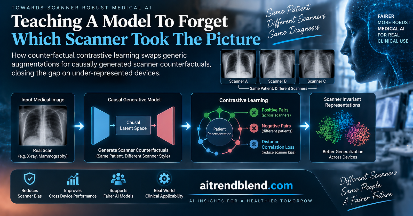
- Researchers at Imperial College London replaced generic image augmentations in contrastive pretraining with causally generated counterfactuals showing the same patient as if scanned on a different device.
- The method works with any contrastive objective, demonstrated on both SimCLR and DINO-v2, because it only changes how positive pairs are formed.
- Gains concentrate exactly where they are needed, on scanners under-represented during training and in low label settings, reaching 4 to 6 percent ROC-AUC on an external mammography dataset.
- A controlled baseline confirms the pairing mechanism is doing the work, not simply the extra synthetic images, and a scanner classifier probing the features drops from 85 percent to 68 percent accuracy.
- Swapping the intervention variable from scanner to biological sex reduced performance disparities between male and female subgroups, though one dataset showed a levelling down effect.
Not Medical Advice
This article explains a published research paper. It is not medical advice, a diagnostic tool, or a treatment recommendation. Questions about mammography screening, breast density, or chest imaging should be directed to a qualified radiologist or physician rather than based on anything summarized here.
Why contrastive learning borrowed the wrong augmentations
Contrastive pretraining has become a standard way to squeeze value out of the enormous piles of unlabelled medical scans sitting in hospital archives. The idea is straightforward. Take an image, produce two different views of it, and train an encoder to map both views to nearby points in feature space while pushing unrelated images apart. The model never sees a diagnosis label. It just learns what counts as the same underlying thing versus a different thing.
Everything hinges on how those two views get made. The standard recipe, inherited from SimCLR and the natural image literature it grew out of, applies random crops, flips, colour jitter, and blur. The implicit message to the model is that none of those changes affect meaning, so learn to ignore them. For photographs of cats and cars, that works well. A cat under different lighting is still a cat.
Medical imaging breaks this assumption in a specific way. The variations that actually matter to ignore are not brightness shifts or crops. They are the compound effects of different acquisition hardware, different detector calibration, different post processing software running inside the scanner. A mammogram from a Hologic Selenia Dimensions and one from a GE Senographe Pristina differ in texture, contrast falloff, and edge characteristics in ways no combination of handcrafted colour transforms replicates. Meanwhile the differences that carry clinical meaning, subtle tissue patterns, are often smaller in magnitude than the scanner differences.
The consequence is a model that quietly encodes which machine took the picture into its representation, because nothing in training told it not to. You can see this directly in the paper’s feature space visualizations, where standard contrastive embeddings cluster by scanner rather than by anatomy.
The counterfactual move
Instead of trying to approximate scanner variation with handcrafted transforms, the authors generate it properly. They train a causal image generation model that can answer a specific what if question, namely how would this exact mammogram look if it had been acquired on a different device? Then they pair the real image with its counterfactual and hand that pair to the contrastive objective as a positive pair.
The framing here is causal rather than merely generative, and the distinction matters. A Structural Causal Model separates observed variables from the unobserved noise that produces everything the model does not explicitly account for. Generating a counterfactual follows three steps. Abduction infers the noise consistent with the observed image. Intervention changes one variable, in this case the scanner indicator, through the do operator. Prediction regenerates the image under the modified model while holding the inferred noise fixed. That last part is what preserves patient identity. The anatomy, the tissue pattern, the lesion if there is one, all come from the fixed noise term, while only the device characteristics change.
A useful theoretical note underpins all of this. Prior work has shown that contrastive learning provably separates content from style, provided the augmentations faithfully capture realistic style changes. Standard augmentations are a crude approximation of that condition. Counterfactual generation is a much more direct attempt to satisfy it.
The generation model itself is a hierarchical variational autoencoder rather than a diffusion model, a choice the authors defend on two grounds. It is far cheaper to train and sample from, and diffusion models have a documented tendency not to preserve identity reliably, which would be fatal here. If the counterfactual changes the anatomy along with the scanner, the contrastive objective learns to discard anatomical information, which is precisely the opposite of what you want.
Worth Remembering
The causal graph used here is deliberately minimal, containing only the scanner variable. That matters more than it first appears. Because no downstream task label enters the graph, the generation step stays fully unsupervised, preserving the whole point of self supervised pretraining.
Two objectives, one pairing strategy
Applying this to SimCLR produces CF-SimCLR. For each image, the authors sample a target domain at random from all available scanners, generate the corresponding counterfactual, and pair it with the real image. If the sampled domain happens to be the original one, the real image is simply reused. The standard augmentation pipeline still runs on top of that cross domain pair, adding view diversity. Nothing else about SimCLR changes.
Extending to DINO-v2 shows the method is not tied to one objective. DINO-v2 works with multiple crops rather than two views, generating two global crops and eight local ones, and trains a student network to match a momentum updated teacher. In CF-DINO, one global crop comes from the real image and one from its counterfactual, and the local crops split four and four. The model is then pushed toward consistent representations across every one of those views, which now span two scanners instead of one.
This portability is the strongest structural argument for the approach. It touches only the positive pair construction step, so it drops into whatever contrastive framework a team already runs.
The baseline that makes the result credible
There is an obvious objection to all of this. Counterfactual contrastive learning trains on roughly twice as many images as the baseline, since every real image now has a synthetic partner. Maybe the gains just come from having more data, and the causal story is decoration.
The authors anticipated this and built the control that answers it. SimCLR+ and DINO+ train on the exact same expanded dataset, real images plus all generated counterfactuals, but treat every image as an independent sample and apply standard contrastive pairing. Same data, same compute, only the pairing mechanism differs. This is the comparison that separates the mechanism from the volume.
What the numbers show
Evaluation spans two modalities and five public datasets. For chest radiography, PadChest provides pretraining data from two scanners, with pneumonia detection evaluated in distribution on PadChest itself and out of distribution on RSNA Pneumonia and CheXpert. For mammography, the EMBED dataset supplies over 300,000 scans from six devices, with one scanner held out entirely, and breast density prediction evaluated in distribution plus externally on VinDR-Mammo from Vietnam. Encoders are ResNet-50 for the SimCLR variants and ViT-Base for the DINO-v2 variants, and every model is finetuned on real data only.
The EMBED scanner imbalance is the whole reason this dataset was chosen. Roughly 90 percent of it comes from a single device, with the remaining five scanners sharing what is left. That is a realistic picture of a hospital fleet and an ideal stress test.
| Setting | Objective | Scanner or dataset | Labels | Gain over baseline |
|---|---|---|---|---|
| Pneumonia, in distribution | CF-SimCLR | PadChest Imaging | 3,249 | 2.5 percent ROC-AUC |
| Pneumonia, in distribution | CF-SimCLR | PadChest Phillips | 3,249 | 0.6 percent ROC-AUC |
| Breast density, in distribution | CF-SimCLR | Clearview CSm | 2,230 | 3 percent ROC-AUC |
| Breast density, in distribution | CF-SimCLR | Senographe Pristina | 2,230 | 1.3 percent ROC-AUC |
| Breast density, external | CF-SimCLR | VinDR-Mammo | 560 to 1,121 | 4 to 6 percent ROC-AUC |
| Breast density, in distribution | CF-DINO | Senograph 2000D | 2,223 | 4 percent ROC-AUC |
| Breast density, external | CF-DINO | VinDR PlanMed Nuance | 1,121 | 6 percent ROC-AUC |
| Pneumonia, external | CF-DINO | RSNA Pneumonia | 2,158 | 3.5 percent ROC-AUC |
Gains land where they should
The pattern across every table is consistent and worth stating plainly. Improvements are largest on scanners that were under-represented during pretraining, largest when labelled data for the downstream task is scarce, and they shrink toward zero as labels become plentiful. That last part is not a weakness, it is exactly what the theory predicts. With 223,000 labelled EMBED samples available for finetuning, the classifier can learn a separate decision boundary for each scanner even if the representation clusters by device. Domain aligned representations only buy you something when you lack the data to paper over the misalignment.
The external dataset results deserve particular attention. Neither the encoder nor the counterfactual generation model ever saw VinDR-Mammo, RSNA Pneumonia, or CheXpert during training. The gains of 4 to 6 percent on VinDR with a few hundred labels come from a representation that generalizes to acquisition domains it was never shown, which is a stronger claim than performing well on held out scanners from the same institution.
One result runs the other way and the paper reports it rather than burying it. On CheXpert with linear probing, CF-DINO slightly underperforms standard DINO at the 25 percent and 100 percent label levels. The authors note CheXpert labels are derived by natural language processing from reports and are generally of lower quality than the expert annotated RSNA labels, which shows up as a performance drop for every model on that dataset, not just theirs.
The pairing mechanism, not the extra data
Against the SimCLR+ and DINO+ controls, the counterfactual pairing wins consistently. CF-SimCLR outperformed SimCLR+ across every experimental setting tested, and the same held for CF-DINO against DINO+ in most comparisons. More telling than the wins is the character of the difference. Simply adding synthetic images to the training set produced unstable gains, helping on some domains while performing no better than baseline on others. The explicit pairing produced consistent improvement, with the starkest gap appearing on the under-represented scanners.
The cleanest evidence comes from probing the feature space directly. The authors trained a scanner classifier on the frozen features from each encoder, balancing the scanner distribution and running five fold cross validation with a small dimensionality reduction step before logistic regression. Standard SimCLR features let a classifier identify the scanner with 85 percent balanced accuracy, and SimCLR+ features actually made it slightly easier at 87 percent. CF-SimCLR features dropped that to 68 percent.
The more domain agnostic image representations are, the bigger the expected improvement in terms of robustness to acquisition shift. Roschewitz et al., Medical Image Analysis, 2025
That 85 to 68 percent drop is the mechanism made visible. The information about which machine took the picture is measurably harder to recover from the counterfactually trained representation, which is the entire design goal stated as a number.
How good do the counterfactuals need to be
A reasonable worry about any method built on generated images is that it inherits every flaw of the generator. The authors ran an ablation comparing three generation models of deliberately varying quality, measured on established axiomatic soundness metrics.
| Generation model | Effectiveness on scanner intervention | Reversibility | Composition |
|---|---|---|---|
| HVAE trained one epoch | 49 percent | 0.001 | 8e-12 |
| HVAE trained 20 epochs | 77 percent | 0.002 | 5e-12 |
| HVAE with counterfactual finetuning | 96 percent | 0.004 | 5e-12 |
Effectiveness measures whether the generated counterfactual actually obeys the requested intervention, tested by whether a scanner classifier trained on real data assigns it the target scanner. Reversibility and composition measure identity preservation, whether applying and undoing an intervention returns the original image. Notice that effectiveness varies enormously across the three models while reversibility and composition stay strong throughout. All three preserve patient identity well, which is the property that actually matters most for contrastive pairing.
The downstream results follow sensibly. Even the weakest generator, at 49 percent effectiveness, produced an encoder that matched or beat the standard SimCLR baseline, particularly on under-represented scanners and in low label settings. Improving effectiveness helped most where the counterfactuals were hardest to generate, with the fully finetuned model delivering 4 percent, 2 percent, 0.5 percent, and 1.8 percent ROC-AUC improvements on the extremely rare Senographe Pristina scanner across different label levels. But the returns diminish. On Clearview CSm, pushing effectiveness from 85 to 97 percent produced no meaningful downstream change. The authors conclude that around 80 percent scanner effectiveness is sufficient, which is a practically useful threshold for anyone deciding how much to invest in the generator.
Beyond scanners
The framework does not care what variable you intervene on. To demonstrate this, the authors swapped scanner counterfactuals for biological sex counterfactuals in the pair generation step, aiming to reduce performance disparities between male and female patients on pneumonia detection.
The standard SimCLR baseline performed worse on female patients across all three chest X-ray datasets. Pairing each image with its sex counterfactual improved female subgroup performance by 2 percent ROC-AUC on PadChest with 3,249 labels, 5 percent on CheXpert with 1,381 labels, and 3 percent on CheXpert with 3,452 labels. On PadChest and CheXpert, male subgroup performance also edged up slightly, meaning the disparity closed without anyone losing ground.
On RSNA Pneumonia it worked differently and the paper says so. The gap closed, but partly because male subgroup performance dropped slightly. The fairness literature calls this levelling down, and it is a real concern rather than a technicality. A method that equalizes outcomes by making the better served group worse off is not straightforwardly an improvement, and reporting it rather than highlighting only the favourable datasets is to the authors’ credit.
What this costs to run
Adding a generative model to a pretraining pipeline sounds expensive. The numbers say otherwise, mostly because contrastive pretraining is already so costly that the generator disappears into the noise.
The hierarchical variational autoencoder needed 20 epochs on EMBED, roughly 250,000 steps, and fit in 20 GB of GPU memory. Generating over a million counterfactual mammograms at 224 by 224 resolution took under seven hours on a single consumer grade RTX-3090. Compare that to the contrastive pretraining it feeds, where each SimCLR model ran for 450 epochs on EMBED or 1,000 on PadChest requiring two 46 GB GPUs, and DINO needed six 46 GB GPUs for a batch size of 300. The generator is a rounding error against that, and it runs once rather than per experiment.
The clinical translation gap
Nothing here is a deployed clinical system, and the tasks chosen are research proxies rather than diagnostic endpoints. Breast density prediction matters clinically as an input to risk modelling, and pneumonia detection from chest X-rays is a real task, but both are evaluated here as classification benchmarks against retrospective public datasets rather than in prospective clinical use.
The more relevant translation question is about where this method sits in a deployment pipeline. It improves the pretrained representation, which is upstream of everything a hospital would actually validate. A system built on a CF-SimCLR encoder would still need its own downstream training, its own clinical validation, and its own regulatory pathway. What the method plausibly changes is how much labelled data that downstream step requires, and how evenly the resulting system performs across the machines in a given department, which are meaningful practical benefits rather than diagnostic claims.
There is also a workflow prerequisite worth naming. Training the counterfactual generator requires scanner metadata attached to every image, which the authors note was conveniently available in PadChest. Institutions where acquisition metadata is missing, inconsistent, or stripped during anonymization would need to solve that before any of this becomes usable.
Honest limitations
The authors are direct about several constraints, and a few more are worth adding.
Gains are bounded by generation quality. The ablation shows the method degrades gracefully rather than catastrophically when the generator is weak, but it also shows the biggest wins on the rarest scanners depend on the generator handling those rare scanners well, which is precisely where generation is hardest because training data for them is scarce. That circularity is real, even if the results suggest it is not fatal.
Choosing the intervention variable is a human judgment call, not something the method determines. The paper lays out a sensible process, analyse the data for likely sources of bias, discuss candidate variables with domain experts, build the causal graph, then generate. But a team that picks the wrong variable will produce a model invariant to something that did not matter while remaining sensitive to something that did.
The causal graph used throughout is minimal, containing one or two variables, with everything else absorbed into the exogenous noise. The authors justify this because they only intervene on one variable at a time, and it keeps the generation unsupervised. Whether richer graphs with interacting variables behave as well is explicitly left to future work.
The levelling down result on RSNA is a genuine limitation for anyone considering the subgroup application. Reducing disparity is not automatically the same as improving care, and this method does not come with a guarantee about which direction the equalization runs.
Finally, two of the five authors report employment relationships with commercial medical imaging companies, and one author reports funding from Google, all disclosed in the paper. This does not undermine results built on public datasets with published code, but it is context a reader should have.
Where this goes next
The most obvious extension is combining multiple intervention variables in a single causal graph, which the authors flag directly. Real deployment settings rarely face just one distribution shift, and a model that needs robustness to both scanner and patient demographics currently requires choosing between them.
The compatibility angle is also worth noting. This approach does not compete with generative data augmentation methods that synthesize additional examples for under-represented classes or subgroups, because counterfactual generation can be applied to synthetic images too. The controlled comparison against SimCLR+ shows that counterfactual pairing changes the organisation of the embedding space rather than merely enriching the training distribution, which suggests the two strategies address different problems and could stack.
And as image synthesis continues improving, the ceiling on this method rises with it. The ablation makes that dependency explicit, showing a clear if diminishing relationship between counterfactual effectiveness and downstream performance on the hardest domains.
Conclusion
The idea at the centre of this paper is narrow and well executed. Contrastive learning works by telling a model which differences to ignore, that message is delivered entirely through how positive pairs get constructed, and medical imaging has been using a message borrowed from natural photographs that does not describe its actual nuisance variation. Generating the real nuisance variation causally and pairing across it is a direct fix.
What makes the result convincing is not the headline gains but the control design. The SimCLR+ comparison isolates the pairing mechanism from the extra data. The scanner classifier probe turns the abstract claim about domain invariant features into a measured drop from 85 to 68 percent. The generation quality ablation maps out how much the method depends on its generator and where that dependency stops mattering. Each of those answers a question a skeptical reader would raise.
The transferable lesson runs past medical imaging. Any self supervised setup where the augmentation pipeline is a proxy for real world variation is making an assumption that can be checked and, where it fails, replaced with generated variation that actually matches. Satellite imagery across sensors, industrial inspection across camera setups, audio across recording conditions all have the same shape of problem.
The limitations are real and stated. Gains depend on generator quality, the intervention variable is a human choice, the causal graphs are minimal, and one subgroup experiment showed levelling down. But the code is public, the datasets are public, and the method only touches one step of an existing pipeline. That combination makes this unusually easy for another team to test on their own fleet of scanners, which is where the claim will actually be settled.
Reference implementation
The interesting code here is the pair construction, not the contrastive loss, which is unchanged from standard SimCLR. The version below implements counterfactual pair sampling, the two baseline strategies for comparison, and the NT-Xent objective they all feed into.
import random
from typing import Dict, List, Optional

import torch
import torch.nn as nn
import torch.nn.functional as F
from torch.utils.data import Dataset


# ---------------------------------------------------------------------------
# 1. Counterfactual bank. In the paper, all domain counterfactuals are
#    pre-generated offline by the causal model, then looked up during training.
# ---------------------------------------------------------------------------
class CounterfactualBank:
    """Maps (image_id, target_domain) to a pre-generated counterfactual."""

    def __init__(self, domains: List[str]):
        self.domains = domains
        self.store: Dict[tuple, torch.Tensor] = {}

    def add(self, image_id: str, domain: str, image: torch.Tensor):
        self.store[(image_id, domain)] = image

    def get(self, image_id: str, domain: str) -> Optional[torch.Tensor]:
        return self.store.get((image_id, domain))


# ---------------------------------------------------------------------------
# 2. The three pairing strategies being compared
# ---------------------------------------------------------------------------
class ContrastivePairDataset(Dataset):
    """
    mode = "simclr"    two augmented views of the same real image
    mode = "simclr+"   same expanded pool, but counterfactuals are treated as
                       independent samples, so pairs never cross domains
    mode = "cf-simclr" one view from the real image, one from a counterfactual
                       drawn from a randomly sampled target domain
    """

    def __init__(self, records, bank: CounterfactualBank, augment, mode="cf-simclr", seed=0):
        self.records = records       # each has .image, .image_id, .domain
        self.bank = bank
        self.augment = augment
        self.mode = mode
        self.rng = random.Random(seed)

        if mode == "simclr+":
            # Flatten real images and every counterfactual into one pool.
            self.pool = []
            for r in records:
                self.pool.append(r.image)
                for d in bank.domains:
                    cf = bank.get(r.image_id, d)
                    if cf is not None:
                        self.pool.append(cf)
        else:
            self.pool = None

    def __len__(self):
        return len(self.pool) if self.pool is not None else len(self.records)

    def __getitem__(self, idx):
        if self.mode == "simclr+":
            base = self.pool[idx]
            return self.augment(base), self.augment(base)

        record = self.records[idx]

        if self.mode == "simclr":
            return self.augment(record.image), self.augment(record.image)

        # cf-simclr: sample a target domain uniformly from all available ones.
        target_domain = self.rng.choice(self.bank.domains)
        if target_domain == record.domain:
            # No domain change needed, reuse the real image.
            partner = record.image
        else:
            partner = self.bank.get(record.image_id, target_domain)
            if partner is None:
                partner = record.image

        # The standard augmentation pipeline still runs on top of the pair.
        return self.augment(record.image), self.augment(partner)


# ---------------------------------------------------------------------------
# 3. NT-Xent loss, unchanged from standard SimCLR
# ---------------------------------------------------------------------------
def nt_xent_loss(z_i: torch.Tensor, z_j: torch.Tensor, temperature=0.1) -> torch.Tensor:
    batch_size = z_i.shape[0]
    z = torch.cat([z_i, z_j], dim=0)
    z = F.normalize(z, dim=1)

    similarity = z @ z.T / temperature
    # Mask out self-similarity on the diagonal.
    mask = torch.eye(2 * batch_size, dtype=torch.bool, device=z.device)
    similarity = similarity.masked_fill(mask, float("-inf"))

    # Positive partner for index k is k+batch_size, and vice versa.
    targets = torch.cat([
        torch.arange(batch_size, 2 * batch_size),
        torch.arange(0, batch_size),
    ]).to(z.device)

    return F.cross_entropy(similarity, targets)


# ---------------------------------------------------------------------------
# 4. Encoder plus projection head
# ---------------------------------------------------------------------------
class ContrastiveModel(nn.Module):
    def __init__(self, encoder: nn.Module, feature_dim=2048, projection_dim=128):
        super().__init__()
        self.encoder = encoder
        self.projector = nn.Sequential(
            nn.Linear(feature_dim, feature_dim),
            nn.ReLU(inplace=True),
            nn.Linear(feature_dim, projection_dim),
        )

    def forward(self, x):
        h = self.encoder(x).flatten(1)
        return h, self.projector(h)


# ---------------------------------------------------------------------------
# 5. Domain separability probe. This is the measurement that turned the
#    paper's abstract claim into a number (85 percent down to 68 percent).
# ---------------------------------------------------------------------------
@torch.no_grad()
def extract_features(model, loader, device):
    model.eval()
    feats, domains = [], []
    for images, domain_labels in loader:
        h, _ = model(images.to(device))
        feats.append(h.cpu())
        domains.append(domain_labels)
    return torch.cat(feats), torch.cat(domains)


def scanner_separability(features: torch.Tensor, domains: torch.Tensor, n_components=16):
    """Balanced accuracy of predicting the scanner from frozen features.
    Lower means the representation carries less acquisition information."""
    from sklearn.decomposition import PCA
    from sklearn.linear_model import LogisticRegression
    from sklearn.model_selection import cross_val_score

    x = PCA(n_components=n_components).fit_transform(features.numpy())
    y = domains.numpy()
    scores = cross_val_score(
        LogisticRegression(max_iter=1000), x, y,
        cv=5, scoring="balanced_accuracy",
    )
    return scores.mean()


# ---------------------------------------------------------------------------
# 6. Smoke test on dummy tensors
# ---------------------------------------------------------------------------
if __name__ == "__main__":
    torch.manual_seed(0)

    class Record:
        def __init__(self, image_id, domain, image):
            self.image_id, self.domain, self.image = image_id, domain, image

    domains = ["selenia", "pristina", "clearview"]
    bank = CounterfactualBank(domains)

    records = []
    for i in range(8):
        img = torch.randn(1, 64, 64)
        records.append(Record(f"img{i}", "selenia", img))
        for d in domains:
            if d != "selenia":
                # Stand-in for a causally generated counterfactual.
                bank.add(f"img{i}", d, img + 0.1 * torch.randn_like(img))

    identity_augment = lambda t: t + 0.01 * torch.randn_like(t)

    for mode in ["simclr", "simclr+", "cf-simclr"]:
        ds = ContrastivePairDataset(records, bank, identity_augment, mode=mode)
        v1, v2 = ds[0]
        print(f"{mode:10s} dataset size {len(ds):3d}  view shapes {tuple(v1.shape)} {tuple(v2.shape)}")

    encoder = nn.Sequential(nn.Conv2d(1, 16, 3, padding=1), nn.AdaptiveAvgPool2d(1))
    model = ContrastiveModel(encoder, feature_dim=16, projection_dim=8)

    batch = torch.randn(4, 1, 64, 64)
    _, z_i = model(batch)
    _, z_j = model(batch + 0.05 * torch.randn_like(batch))
    print(f"NT-Xent loss on dummy batch: {nt_xent_loss(z_i, z_j).item():.4f}")
Left out here is the causal generation model itself, the hierarchical variational autoencoder that produces the counterfactuals, which is substantial enough to warrant its own treatment and is available in the authors’ published repository along with everything needed to reproduce the experiments.
Frequently Asked Questions
What is counterfactual contrastive learning
It is a way of building the positive pairs used in contrastive pretraining. Instead of creating two views of an image with generic augmentations like cropping and colour jitter, it pairs a real image with a causally generated version of that same image as it would appear if acquired on a different scanner. The contrastive objective then learns to treat scanner differences as meaningless.
Why do generic augmentations fail for medical imaging
Augmentation pipelines were developed for natural photographs, where brightness and crop changes approximate real variation well. In medical imaging the dominant nuisance variation comes from acquisition hardware, detector calibration, and scanner post processing software, whose combined effect on image appearance is too complex for handcrafted colour and geometry transforms to replicate. Meanwhile the clinically meaningful differences are often subtler than the scanner differences.
Does this work with any contrastive learning method
Yes, because it only changes how positive pairs are formed and leaves the training objective untouched. The paper demonstrates this on two quite different frameworks, SimCLR with a ResNet-50 encoder and DINO-v2 with a ViT-Base encoder, and reports improvements with both.
How do we know the gains come from the pairing and not just extra training data
The authors built a control called SimCLR+ that trains on exactly the same expanded dataset of real images plus counterfactuals, but treats every image as an independent sample with standard pairing. Counterfactual pairing outperformed it consistently. A separate probe found that a classifier could identify the scanner from standard SimCLR features with 85 percent balanced accuracy but only 68 percent from counterfactual contrastive features.
How good does the counterfactual generation model need to be
Better than expected is not required. Even a generator with 49 percent effectiveness produced encoders matching or beating the baseline. Improvements did increase with generation quality, particularly on the rarest scanners, but with diminishing returns. The authors conclude that scanner effectiveness above 80 percent is satisfactory.
Can this method reduce bias across patient subgroups as well as scanners
The framework accepts any intervention variable, and the paper tested biological sex counterfactuals to reduce male and female performance disparities on pneumonia detection. Female subgroup performance improved by 2 to 5 percent ROC-AUC depending on the dataset and label budget. On one dataset the disparity closed partly because male performance dropped slightly, a levelling down effect the authors report explicitly.
Read the full open access paper for every per scanner result, the feature space visualizations, and the complete ablation, or clone the authors’ code.
This analysis is based on the published paper and an independent evaluation of its claims.
Pingback: Revolutionary AI Breakthrough: Non-Contrast Tumor Segmentation Saves Lives & Avoids Deadly Risks - aitrendblend.com