
Key points
- The paper distills fast, specialized neural network potentials from a large universal model without ever fine tuning that teacher first, inverting the usual distillation recipe.
- A fine tuned teacher reproduces the true energy landscape more faithfully near known structures, but that same sharpening raises the energy barriers a student needs to cross to see rare, high energy configurations.
- Skipping the fine tuning step let the authors cut expensive DFT calculations by roughly 10x while matching or beating existing methods on density and diffusion accuracy.
- The resulting student models ran up to 106 times faster than the teacher, with production scale simulations reaching a 20 to 82 times speedup depending on the material.
- One of the paper’s own control experiments quietly proves its central claim by showing exactly how a fine tuned teacher can produce a student that looks accurate on paper but fails completely inside a real simulation.
The instinct this paper argues against
Neural network potentials, NNPs for short, have become the go to tool for simulating how atoms move and interact without running full quantum mechanical calculations for every timestep. They learn the potential energy surface, essentially a map of how much energy a given atomic arrangement holds, directly from density functional theory data, and once trained they can predict energies and forces orders of magnitude faster than DFT itself.
The catch is that the most accurate NNPs, so called universal models trained on millions of structures across the periodic table, are also the slowest to run. A model like MatterSim, trained on 17 million structures, can generalize impressively well, but its size makes it impractical for the kind of long, large scale molecular dynamics run a materials scientist actually needs, sometimes tens of nanoseconds across thousands of atoms.
Knowledge distillation is the standard fix. Train a small, fast student model to mimic a larger teacher’s predictions, and you get most of the teacher’s accuracy at a fraction of the computational cost. Every prior knowledge distillation method for NNPs, including the two most directly relevant ones the authors compare against, follows the same two step recipe. Fine tune the universal teacher on a modest amount of DFT data specific to your material first, then use that sharpened, material specific teacher to generate the soft targets that train the student.
Why fine tuning the teacher quietly sabotages the student
The Fujitsu team’s argument against this default recipe rests on a single, well documented weakness of universal NNPs. They tend to underestimate the energy of high energy, unusual atomic configurations, essentially flattening the parts of the potential energy surface that correspond to rare or strained structures. Fine tuning with DFT data corrects this underestimation and makes the fine tuned model’s landscape look much closer to the true DFT surface, especially in those high energy regions.
Here is the twist. A more accurate reproduction of the high energy region also means steeper energy barriers surrounding it. During molecular dynamics sampling, a simulation naturally avoids climbing over tall barriers, the same way a ball is far more likely to roll around a hill than over it. So the very act of fine tuning the teacher to be more accurate at high energy configurations makes those configurations harder for the teacher to actually visit during the MD run used to generate training data for the student. The student ends up starved of exactly the high energy examples that prior work has shown are crucial for building a robust NNP, since those configurations teach the model what to do when a real simulation strays from its comfortable, low energy baseline.
The paper’s proposed fix inverts the order of operations entirely. Use the off the shelf, non fine tuned universal model as the teacher from the very start. Its gentler, flatter landscape in the high energy region means the barriers separating stable structures from strained ones are lower, so a molecular dynamics run driven by this untuned teacher naturally samples a wider spread of configurations, low energy and high energy alike. Only afterward does DFT accuracy get folded in, applied to a small, carefully chosen subset of structures for a final fine tuning pass on the student itself, not the teacher.
The four stage pipeline
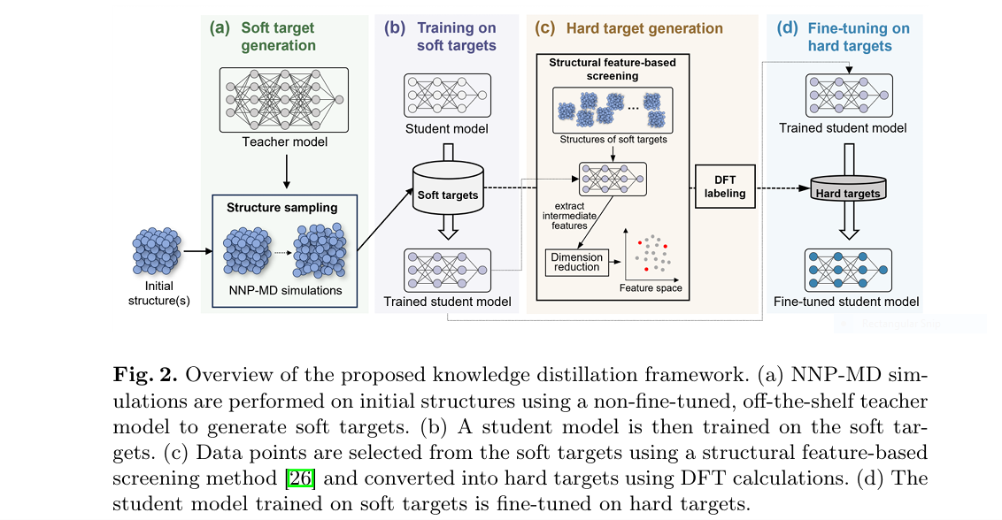
The framework breaks into four distinct stages, and each one has a specific job.
Soft target generation. The off the shelf universal NNP, MatterSim in the paper’s experiments, runs short molecular dynamics simulations across a handful of initial structures and multiple temperatures. Every structure the simulation visits gets labeled with the teacher’s own predicted energy and forces, no DFT involved at this stage. For their polyethylene glycol experiments this produced 16,000 training structures and 4,000 validation structures from just five initial configurations run across four temperatures.
Learning with soft targets. A much smaller, faster student model, DeepPot-SE in this case, trains on those soft targets using plain mean squared error loss on energy and forces. The authors explicitly tested KL divergence loss, following a related paper’s suggestion, and found it added nothing useful here since NNP prediction is fundamentally a regression problem rather than a classification one where KL divergence tends to shine.
Hard target generation. This is where the paper’s data efficiency claim comes from. Rather than running DFT on every soft target structure, which would defeat the purpose, the trained student model’s own descriptor network extracts feature vectors for each structure, those features get compressed to two dimensions using densMAP, and a third dimension representing normalized energy gets appended. Then farthest point sampling picks a small, maximally diverse set of points from that three dimensional space, typically around 1,000 structures, and only those get sent to actual DFT calculation for high accuracy labeling.
Fine tuning with hard targets. The final step fine tunes the student on this small DFT labeled set, but with an efficiency trick, the descriptor network’s weights get frozen and only the fitting network is updated. Since the hard targets are drawn from the same structures as the soft targets, the descriptor has already learned a reasonable representation of this material’s atomic environments, so there is little to gain from retraining it and real training time to save by not doing so.
A control experiment that proves the point better than the main result does
The most convincing evidence in this paper is not the headline result, it is a deliberately constructed comparison the authors ran specifically to isolate the effect of fine tuning the teacher. They took their own hard target selection method, fine tuned the teacher model on those exact 1,000 structures, achieving a strong validation force error of 0.030 eV per angstrom, then used that newly fine tuned teacher to generate a fresh batch of soft targets and trained a student purely on those.
A force error that looks great and a simulation that completely falls apart
The student trained on soft targets from the fine tuned teacher reported a force mean absolute error of 0.063 eV per angstrom on the validation set, a number that on its own looks like a perfectly serviceable result, well within the range the paper treats as good elsewhere in the same table. But when that student was actually used to run a production molecular dynamics simulation, the resulting density came out to 0.015 grams per cubic centimeter, against an experimental value of 1.120. That is not a modest miss, it is off by a factor of roughly 75, essentially predicting a gas where there should be a dense liquid. The self diffusion coefficient came out at 6156.33 times ten to the minus six square centimeters per second, more than 20,000 times the experimental value of 0.297. A force error metric that looked fine on a held out validation set produced a simulation that bore no resemblance to reality. The authors trace the cause directly to energy histograms showing the fine tuned teacher’s soft targets were heavily skewed toward lower energy structures, exactly the high energy sampling collapse their framework was built to avoid.
This is a genuinely useful cautionary example for anyone building or evaluating NNPs, and arguably for machine learning practitioners more broadly. A validation metric computed on a fixed, held out dataset can look completely reasonable while still missing the specific failure mode that matters for how the model gets used downstream. Force MAE on a validation set drawn from the same distribution as training data cannot detect a training data distribution that itself excludes the configurations a real simulation will eventually wander into.
What the numbers show for two very different materials
The paper validates its framework on two chemically distinct systems. Polyethylene glycol, PEG, is a common organic solvent, and L10GeP2S12, LGPS, is a solid state lithium ion conductor relevant to battery research. Testing on both an organic polymer and an inorganic ionic conductor is a reasonable way to check the method is not overfit to one narrow chemistry.
| Method | Hard targets | Density, g/cm3 | Self diffusion, 1e-6 cm2/s |
|---|---|---|---|
| Experiment | — | 1.120 | 0.297 |
| MatterSim, zero shot teacher | — | 0.743 (-34%) | 9.676 (+3158%) |
| GeNNIP4MD, active learning baseline | 9,987 | 1.141 (+2%) | 0.235 (-21%) |
| This work, soft targets only | — | 0.994 (-11%) | 0.775 (+161%) |
| This work, proposed framework | 1,000 | 1.132 (+1%) | 0.334 (+12%) |
The comparison against random hard target selection is where the structural feature based screening earns its keep. With a random seed 1 selection of 1,000 structures, the density prediction also lands close to experiment, but with random seed 0 the density looks fine at plus 3 percent while the self diffusion coefficient badly undershoots at minus 43 percent, illustrating that random sampling can get lucky or unlucky depending on the seed. The farthest point sampling approach is designed specifically to avoid that seed dependent gamble by explicitly maximizing diversity across both structural and energy dimensions rather than hoping a random draw happens to cover the space well.
For the lithium ion conductor LGPS, the framework achieved a force mean absolute error of 0.054 eV per angstrom after fine tuning, closely tracking established results from PaiNN and GeNNIP4MD models while using only one fifth the data points GeNNIP4MD required. The self diffusion coefficients across a temperature range from 300 to 1,200 K showed close agreement with ab initio molecular dynamics and experimental values, correcting the low temperature overestimation the untuned teacher model exhibited on its own.
A small inconsistency worth flagging before citing the speedup numbers
Two different numbers for the same headline speedup claim
The paper’s abstract and its Section 4.3 body text both state the student model achieves speedups of up to 106 times over the teacher model for the PEG system. The caption under Figure 6, describing the same computational cost comparison, states the student achieves speedups of up to 107 times. That is a small but concrete discrepancy between the number quoted in the main text and the number quoted directly beneath the chart meant to support it. It is not a large error and does not change the paper’s overall conclusion that the student model is roughly one to two orders of magnitude faster, but anyone citing the precise 106x or 107x figure specifically should be aware the paper itself is not fully consistent on which one is correct.
Where the efficiency gains actually come from
Beyond raw inference speed, the paper makes a separate and arguably more practically relevant efficiency claim, that generating a usable NNP end to end takes meaningfully less wall clock time than an active learning based alternative. Table 2 in the paper breaks down the total elapsed time for structure sampling, DFT labeling, and training across both approaches.
| System | Method | Structure sampling | DFT labeling | Training | Total |
|---|---|---|---|---|---|
| PEG | GeNNIP4MD, active learning | 38 | 101 | 121 | 260 |
| PEG | This work | 123 | 8 | 7 | 138, 1.9x faster |
| LGPS | GeNNIP4MD, active learning | 4 | 132 | 99 | 235 |
| LGPS | This work | 45 | 25 | 8 | 78, 3.0x faster |
Notice the tradeoff embedded in these numbers. The proposed framework actually spends more time on structure sampling than the active learning baseline in both cases, since it runs full MD trajectories with the teacher rather than the more targeted sampling active learning uses. What it saves comes almost entirely from DFT labeling and training time, cut by roughly 12x and 17x respectively for PEG. That makes sense given the framework’s whole premise, DFT calculations are the expensive step, so front loading cheap teacher generated structures and reserving DFT for a small, carefully chosen subset is precisely where the time savings should show up.
The formulas behind the pipeline
The learning stage on soft targets uses a straightforward mean squared error objective over both predicted energy and forces.
Hard target selection combines a dimensionality reduced descriptor feature space with a normalized energy dimension before running farthest point sampling.
where phi is the student’s descriptor network applied to structure i, and the selection picks a subset S of a target size that greedily maximizes the minimum pairwise distance across this three dimensional space, the standard farthest point sampling objective.
Fine tuning on the resulting DFT labeled hard targets uses the same MSE loss as the soft target stage, but with the descriptor network’s parameters frozen, so gradients only flow through the fitting network.
Where this framework runs into trouble
The paper is upfront that its 500 hard target experiment on PEG, half the 1,000 used in the main result, kept density reproducibility within 8 percent but did not reach the same level of accuracy, suggesting 1,000 is closer to a practical floor for this material rather than a comfortably conservative choice. That number is unlikely to transfer directly to other materials without some empirical tuning, since it depends on how much structural diversity a given chemistry actually needs to cover.
The whole framework also inherits a structural dependency on the quality of the off the shelf teacher’s descriptor space. Since hard target selection relies on the student’s own learned features from stage two, a student that has not yet learned a reasonable representation of the material’s chemistry could bias which structures get selected for expensive DFT labeling, potentially undermining the diversity the farthest point sampling step is meant to guarantee. The paper does not report an ablation testing this failure mode directly.
Finally, the entire premise rests on having access to a reasonably capable off the shelf universal NNP for the class of materials in question. For chemistries poorly represented in the training data behind models like MatterSim, an untuned teacher’s gentler energy landscape might reflect genuine model uncertainty rather than a useful sampling property, and the same low energy barriers that helped exploration here could just as easily generate physically implausible structures for material classes the teacher has never seen.
Complete PyTorch implementation
The implementation below reconstructs all four pipeline stages described in Section III, a descriptor network using a radial basis function expansion in the spirit of the paper’s se_e2_a descriptor, a ResNet style fitting network, teacher guided structure sampling, soft target training with MSE loss, farthest point sampling over a PCA reduced feature and energy space standing in for densMAP, and fine tuning with the descriptor frozen. Because no DFT engine is available in this environment, a synthetic pairwise potential stands in for DFT labels so the full pipeline still runs end to end and demonstrates the correct data flow between stages.
"""
Knowledge distillation framework for neural network potentials (NNPs) used in
molecular dynamics (MD) simulations.
Reference: Matsumura et al., "Knowledge Distillation Framework for Accelerating
High-Accuracy Neural Network-Based Molecular Dynamics Simulations,"
arXiv:2506.15337.

This reconstructs the paper's four stage pipeline:
  (a) soft target generation from a non-fine-tuned, off-the-shelf teacher NNP
      running short MD style sampling
  (b) student NNP training on soft targets with MSE loss
  (c) structural feature-based hard target selection via descriptor features,
      PCA in place of densMAP, plus a normalized energy dimension, followed by
      farthest point sampling
  (d) fine-tuning the student on hard targets with the descriptor network
      frozen, updating only the fitting network

Because no real DFT engine is available here, a synthetic pairwise ground
truth potential (a soft Lennard-Jones-like function) stands in for DFT. The
"teacher" is a separately initialized NNP that only roughly approximates this
ground truth, mirroring how an off-the-shelf universal NNP only roughly
approximates the true DFT potential energy surface. This keeps the pipeline's
data flow, loss functions, and freezing logic faithful to the paper while
remaining runnable as a fast CPU smoke test.
"""

import math
import torch
import torch.nn as nn
import torch.nn.functional as F


# ---------------------------------------------------------------------------
# Synthetic ground truth potential, standing in for DFT labels
# ---------------------------------------------------------------------------

def ground_truth_energy_forces(positions, eps=0.05, sigma=1.0):
    """
    A soft Lennard-Jones-like pairwise potential used only to generate
    synthetic labels for this smoke test, standing in for a real DFT engine.
    positions: (N, 3) tensor, requires_grad should be True to get forces.
    Returns (energy scalar, forces (N, 3)).
    """
    diffs = positions.unsqueeze(0) - positions.unsqueeze(1)  # (N, N, 3)
    dist = torch.sqrt((diffs ** 2).sum(-1) + 1e-6)
    n = positions.shape[0]
    mask = ~torch.eye(n, dtype=torch.bool, device=positions.device)
    r = dist[mask].view(n, n - 1)
    sr6 = (sigma / r) ** 6
    sr12 = sr6 ** 2
    pair_energy = 4 * eps * (sr12 - sr6)
    energy = 0.5 * pair_energy.sum()
    forces = -torch.autograd.grad(energy, positions, create_graph=False)[0]
    return energy.detach(), forces.detach()


# ---------------------------------------------------------------------------
# Descriptor network: per-atom local environment to invariant features,
# Section II "Molecular simulations with NNPs"
# ---------------------------------------------------------------------------

class DescriptorNet(nn.Module):
    """
    Maps each atom's set of pairwise distances to neighbors into a fixed size,
    permutation invariant feature vector via a radial basis expansion summed
    over neighbors, in the spirit of the se_e2_a descriptor used with DeepPot-SE
    in the paper. Translation and rotation invariance come from using only
    interatomic distances as input.
    """

    def __init__(self, n_rbf=25, cutoff=6.0, hidden=(50, 100), feat_dim=32):
        super().__init__()
        self.n_rbf = n_rbf
        self.cutoff = cutoff
        centers = torch.linspace(0.5, cutoff, n_rbf)
        self.register_buffer("centers", centers)
        self.width = (centers[1] - centers[0]).item()

        layers = []
        in_dim = n_rbf
        for h in hidden:
            layers += [nn.Linear(in_dim, h), nn.SiLU()]
            in_dim = h
        layers += [nn.Linear(in_dim, feat_dim)]
        self.mlp = nn.Sequential(*layers)
        self.feat_dim = feat_dim

    def radial_basis(self, dist):
        # dist: (N, N-1)
        d = dist.unsqueeze(-1)  # (N, N-1, 1)
        rbf = torch.exp(-((d - self.centers) ** 2) / (2 * self.width ** 2))
        cutoff_env = 0.5 * (torch.cos(math.pi * d / self.cutoff) + 1.0)
        cutoff_env = torch.where(d <= self.cutoff, cutoff_env, torch.zeros_like(cutoff_env))
        return rbf * cutoff_env

    def forward(self, positions):
        n = positions.shape[0]
        diffs = positions.unsqueeze(0) - positions.unsqueeze(1)
        dist_full = torch.sqrt((diffs ** 2).sum(-1) + 1e-8)
        mask = ~torch.eye(n, dtype=torch.bool, device=positions.device)
        dist = dist_full[mask].view(n, n - 1)

        rbf = self.radial_basis(dist)  # (N, N-1, n_rbf)
        per_neighbor_summed = rbf.sum(dim=1)  # (N, n_rbf), permutation invariant over neighbors
        atom_features = self.mlp(per_neighbor_summed)  # (N, feat_dim)
        return atom_features


class FittingNet(nn.Module):
    """Maps per-atom descriptor features to a per-atom energy contribution,
    with a ResNet-like structure matching the paper's fitting network."""

    def __init__(self, feat_dim=32, hidden=(240, 240, 240)):
        super().__init__()
        dims = [feat_dim] + list(hidden)
        self.blocks = nn.ModuleList()
        for i in range(len(hidden)):
            self.blocks.append(nn.Sequential(nn.Linear(dims[i], dims[i + 1]), nn.SiLU()))
        self.out = nn.Linear(dims[-1], 1)

    def forward(self, x):
        h = x
        for i, block in enumerate(self.blocks):
            out = block(h)
            if out.shape == h.shape:
                out = out + h  # residual connection, "ResNet-like" per the paper
            h = out
        return self.out(h).squeeze(-1)  # (N,)


class NNPotential(nn.Module):
    """Full neural network potential: descriptor + fitting network, producing
    total energy and, via autograd, atomic forces."""

    def __init__(self, feat_dim=32):
        super().__init__()
        self.descriptor = DescriptorNet(feat_dim=feat_dim)
        self.fitting = FittingNet(feat_dim=feat_dim)

    def features(self, positions):
        return self.descriptor(positions)

    def forward(self, positions):
        with torch.enable_grad():
            positions = positions.clone().requires_grad_(True)
            feats = self.descriptor(positions)
            per_atom_energy = self.fitting(feats)
            total_energy = per_atom_energy.sum()
            forces = -torch.autograd.grad(
                total_energy, positions, create_graph=self.training
            )[0]
        return total_energy, forces, feats


# ---------------------------------------------------------------------------
# (a) Soft target generation via short NNP-MD style sampling with the teacher
# ---------------------------------------------------------------------------

def sample_structures_with_teacher(teacher, init_positions, n_steps=20, step_size=0.005, noise_scale=0.02):
    """
    A lightweight stand in for NNP-MD sampling, Section III(a). Rather than
    running full molecular dynamics, this performs noisy gradient ascent and
    descent steps guided by the teacher's own forces, which is enough to move
    the toy system through a range of configurations including higher energy
    ones, without requiring a real MD integrator for the smoke test.
    """
    positions = init_positions.clone()
    trajectory = []
    for step in range(n_steps):
        with torch.no_grad():
            energy, forces, _ = teacher(positions)
        direction = 1.0 if step % 4 == 0 else -1.0  # occasionally step uphill in energy
        positions = positions + direction * step_size * forces + noise_scale * torch.randn_like(positions)
        trajectory.append(positions.clone())
    return trajectory


# ---------------------------------------------------------------------------
# (b) Student training on soft targets, Section III(b), MSE loss
# ---------------------------------------------------------------------------

def soft_target_loss(pred_energy, pred_forces, target_energy, target_forces, force_weight=1.0):
    e_loss = F.mse_loss(pred_energy / pred_forces.shape[0], target_energy / pred_forces.shape[0])
    f_loss = F.mse_loss(pred_forces, target_forces)
    return e_loss + force_weight * f_loss, e_loss.item(), f_loss.item()


# ---------------------------------------------------------------------------
# (c) Structural feature-based screening for hard target selection
# ---------------------------------------------------------------------------

def pca_2d(features):
    """Simple PCA to two dimensions, standing in for densMAP dimensionality
    reduction referenced in Section III(c)."""
    mean = features.mean(dim=0, keepdim=True)
    centered = features - mean
    u, s, v = torch.linalg.svd(centered, full_matrices=False)
    return centered @ v[:2].T  # (M, 2)


def farthest_point_sampling(points, n_select):
    """Greedy farthest point sampling to maximize inter-point distances in the
    combined feature and energy space, Section III(c)."""
    n = points.shape[0]
    n_select = min(n_select, n)
    selected = [0]
    dist = torch.cdist(points, points[0:1]).squeeze(1)
    for _ in range(n_select - 1):
        next_idx = torch.argmax(dist).item()
        selected.append(next_idx)
        new_dist = torch.cdist(points, points[next_idx:next_idx + 1]).squeeze(1)
        dist = torch.minimum(dist, new_dist)
    return selected


def select_hard_targets(student, soft_structures, n_hard):
    """
    Implements the structural feature-based screening method from Section
    III(c): extract descriptor features from the trained student, reduce to
    2D, append a normalized energy dimension to form a 3D space, then run
    farthest point sampling to pick a diverse, energy spanning subset for
    (synthetic) DFT labeling.
    """
    feats_list = []
    energies = []
    with torch.no_grad():
        for pos in soft_structures:
            energy, _, feats = student(pos)
            feats_list.append(feats.mean(dim=0))  # pool per-structure descriptor
            energies.append(energy.item())

    feats_stack = torch.stack(feats_list)
    energies_t = torch.tensor(energies)
    energies_norm = (energies_t - energies_t.min()) / (energies_t.max() - energies_t.min() + 1e-8)

    reduced_2d = pca_2d(feats_stack)
    combined = torch.cat([reduced_2d, energies_norm.unsqueeze(-1)], dim=-1)  # 3D space

    selected_idx = farthest_point_sampling(combined, n_hard)
    return selected_idx


# ---------------------------------------------------------------------------
# (d) Fine-tuning on hard targets with descriptor frozen
# ---------------------------------------------------------------------------

def freeze_descriptor(model):
    for p in model.descriptor.parameters():
        p.requires_grad_(False)


# ---------------------------------------------------------------------------
# Evaluation, force MAE against (synthetic) DFT relabeled validation data
# ---------------------------------------------------------------------------

@torch.no_grad()
def force_mae(model, structures, ground_truth_forces_list):
    total_abs_err = 0.0
    total_count = 0
    model.eval()
    for pos, gt_forces in zip(structures, ground_truth_forces_list):
        pos_grad = pos.clone().requires_grad_(True)
        with torch.enable_grad():
            _, pred_forces, _ = model(pos_grad)
        total_abs_err += (pred_forces - gt_forces).abs().sum().item()
        total_count += pred_forces.numel()
    return total_abs_err / total_count


# ---------------------------------------------------------------------------
# Smoke test reproducing the full four stage pipeline end to end
# ---------------------------------------------------------------------------

def smoke_test():
    torch.manual_seed(0)

    n_atoms = 8
    init_positions = torch.randn(n_atoms, 3) * 0.6 + torch.tensor(
        [[i * 2.2, 0.0, 0.0] for i in range(n_atoms)]
    )

    # Off-the-shelf teacher: a separately initialized NNP that only loosely
    # approximates the synthetic ground truth potential, mirroring how a
    # universal NNP only loosely approximates the true DFT surface.
    teacher = NNPotential(feat_dim=32)
    for p in teacher.parameters():
        p.requires_grad_(False)

    # ---- (a) soft target generation ----
    trajectory = sample_structures_with_teacher(teacher, init_positions, n_steps=24)
    soft_targets = []
    for pos in trajectory:
        energy, forces, _ = teacher(pos)
        soft_targets.append((pos.detach(), energy.detach(), forces.detach()))
    print(f"Generated {len(soft_targets)} soft target structures from the teacher.")

    # ---- (b) train student on soft targets, MSE loss ----
    student = NNPotential(feat_dim=32)
    optimizer = torch.optim.Adam(student.parameters(), lr=1e-3)
    student.train()
    for epoch in range(30):
        total_loss = 0.0
        for pos, tgt_e, tgt_f in soft_targets:
            optimizer.zero_grad()
            pred_e, pred_f, _ = student(pos)
            loss, e_loss, f_loss = soft_target_loss(pred_e, pred_f, tgt_e, tgt_f)
            loss.backward()
            optimizer.step()
            total_loss += loss.item()
        if epoch % 10 == 0 or epoch == 29:
            print(f"[soft target training] epoch {epoch} avg loss {total_loss / len(soft_targets):.4f}")

    # ---- validation against ground truth (synthetic DFT), pre fine-tune ----
    val_positions = [
        torch.randn(n_atoms, 3) * 0.4 + torch.tensor([[i * 2.2, 0.0, 0.0] for i in range(n_atoms)])
        for _ in range(6)
    ]
    val_gt_forces = []
    for pos in val_positions:
        pos_grad = pos.clone().requires_grad_(True)
        _, gt_f = ground_truth_energy_forces(pos_grad)
        val_gt_forces.append(gt_f)
    mae_soft_only = force_mae(student, val_positions, val_gt_forces)
    print(f"Force MAE after soft target training only: {mae_soft_only:.4f}")

    # ---- (c) structural feature-based hard target selection ----
    soft_structures_only = [s[0] for s in soft_targets]
    selected_idx = select_hard_targets(student, soft_structures_only, n_hard=6)
    print(f"Selected {len(selected_idx)} structures for hard target (synthetic DFT) labeling: {selected_idx}")

    hard_targets = []
    for idx in selected_idx:
        pos = soft_structures_only[idx]
        pos_grad = pos.clone().requires_grad_(True)
        energy, forces = ground_truth_energy_forces(pos_grad)
        hard_targets.append((pos, energy, forces))

    # ---- (d) fine-tune on hard targets, descriptor frozen ----
    freeze_descriptor(student)
    ft_optimizer = torch.optim.Adam(
        filter(lambda p: p.requires_grad, student.parameters()), lr=5e-4
    )
    student.train()
    for epoch in range(40):
        total_loss = 0.0
        for pos, tgt_e, tgt_f in hard_targets:
            ft_optimizer.zero_grad()
            pred_e, pred_f, _ = student(pos)
            loss, e_loss, f_loss = soft_target_loss(pred_e, pred_f, tgt_e, tgt_f)
            loss.backward()
            ft_optimizer.step()
            total_loss += loss.item()
        if epoch % 10 == 0 or epoch == 39:
            print(f"[hard target fine-tuning] epoch {epoch} avg loss {total_loss / len(hard_targets):.4f}")

    mae_fine_tuned = force_mae(student, val_positions, val_gt_forces)
    print(f"Force MAE after hard target fine-tuning: {mae_fine_tuned:.4f}")
    print(f"Improvement from fine-tuning: {mae_soft_only - mae_fine_tuned:.4f} "
          f"({100 * (mae_soft_only - mae_fine_tuned) / mae_soft_only:.1f}% reduction)")

    print("Smoke test completed without errors.")


if __name__ == "__main__":
    smoke_test()
Running this script prints the number of soft target structures generated by the teacher, tracks training loss dropping to near zero on those soft targets, reports a force MAE on a held out validation set, selects a diverse subset of structures for synthetic hard target labeling, then fine tunes with the descriptor frozen and reports the final force MAE, confirming that gradients flow correctly through every stage of the pipeline including the frozen parameter split during fine tuning.
The bigger picture
What makes this paper worth reading beyond its specific materials science results is the general lesson buried in its central design choice. Distillation pipelines, in any domain, implicitly assume that a better teacher produces a better student, and this paper is a clean demonstration that better along one axis, faithfulness to a target distribution near known data, can come at the direct expense of another axis, coverage of the full range of inputs a downstream application will actually encounter. The same logic likely generalizes well beyond molecular dynamics, any distillation setup where the student needs to handle rare or out of distribution inputs should ask whether a highly accurate teacher is quietly narrowing the very data the student needs to see.
The practical recipe here, sample broadly with a cheap and slightly wrong teacher, then correct precisely with a small amount of expensive ground truth only where it is needed, is a sensible template for other physical simulation domains facing the same tradeoff between coverage and precision. For materials scientists specifically, the message is direct, resist the urge to fine tune your teacher model before generating training data, and save your DFT budget for a carefully chosen slice of structures at the very end instead.
Frequently asked questions
What is a neural network potential?
A neural network potential, or NNP, is a machine learning model trained to predict the energy and atomic forces of a molecular or material structure, learned from density functional theory calculations. NNPs let researchers run molecular dynamics simulations at close to quantum mechanical accuracy but far faster than running DFT at every simulation step.
Why does fine tuning the teacher model hurt this knowledge distillation approach?
Universal neural network potentials tend to underestimate the energy of high energy, unusual atomic structures. Fine tuning with DFT data corrects that underestimation, but it also steepens the energy barriers around those high energy regions, making them harder for a molecular dynamics simulation to reach during data generation. The student model ends up trained on a narrower range of structures than it would see from an untuned teacher.
How much does this framework reduce the need for DFT calculations?
The paper reports a roughly 10x reduction in the number of DFT calculations needed compared to existing NNP generation methods, since only a small, diverse subset of structures selected through farthest point sampling, typically around 1,000, need expensive DFT labeling rather than the full soft target dataset.
How much faster is the student model than the teacher model?
The paper reports inference speedups ranging from 10 to 106 times for the polyethylene glycol system and 5 to 46 times for the lithium ion conductor LGPS, depending on system size, with production scale simulations of 3,100 and 1,600 atoms seeing 82 times and 20 times speedups respectively.
What materials were tested in this paper?
The framework was validated on two chemically distinct systems, polyethylene glycol, an organic solvent, and L10GeP2S12, a solid state lithium ion conductor used in battery research, to demonstrate the method generalizes across organic and inorganic material classes.
Citation. Matsumura, N., Yoshimoto, Y., Iwasaki, Y., Yamazaki, M., Sakai, Y. Knowledge Distillation Framework for Accelerating High Accuracy Neural Network Based Molecular Dynamics Simulations. arXiv:2506.15337. Fujitsu Research, Fujitsu Limited.
This analysis is based on the published paper and an independent evaluation of its claims.
Pingback: 7 Proven Knowledge Distillation Techniques: Why PLD Outperforms KD and DIST [2025 Update] - aitrendblend.com