
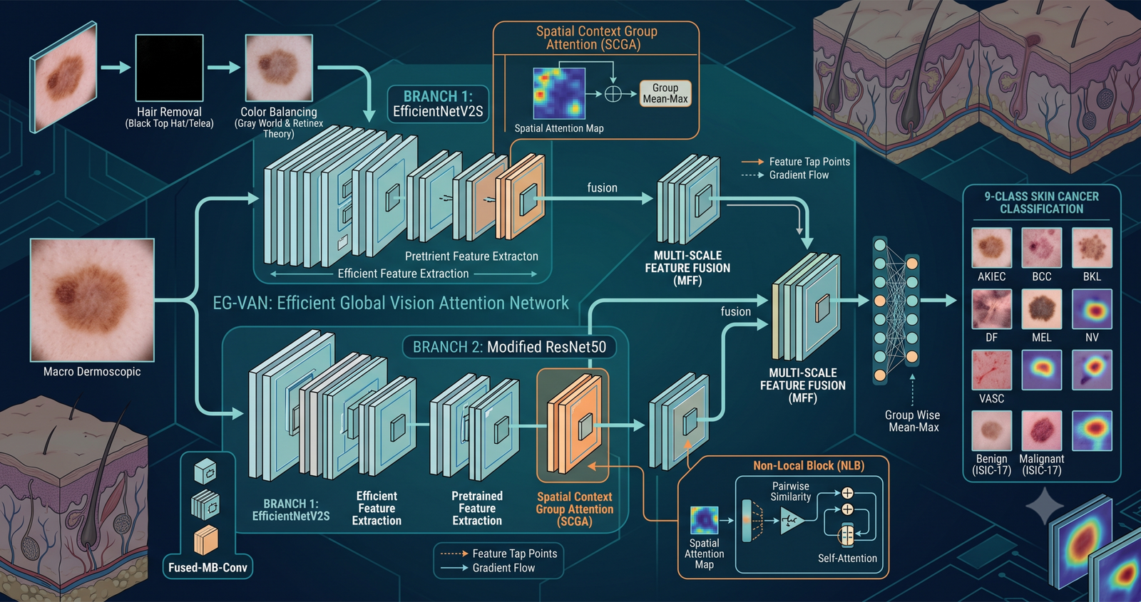
A dermatologist looking at a mole under a dermatoscope is doing something a plain convolutional network struggles with. She is reading fine texture right at the border of the lesion while also holding the whole shape in mind at once, then comparing that combination against a mental library of thousands of prior cases. A paper recently accepted in IEEE Access, written by Adnan Saeed and coauthors from Lahore Leads University, Northeastern University in Shenyang, Prince Sultan University in Riyadh, and Benha University in Egypt, tries to give a EG-VAN neural network something closer to that same two track habit of looking closely and looking broadly at the same time.
Key points
- EG VAN runs two backbones in parallel, EfficientNetV2S and a modified ResNet50, then merges their features at several depths instead of only at the end.
- The ResNet50 branch gets two custom attention pieces, a Spatial Context Group Attention module for local texture and a Non Local Block for long range context.
- A Multi Scale Feature Fusion module blends the two branches using spatial attention and a group wise mean max operation rather than simple concatenation.
- A preprocessing pipeline removes hair with morphological filtering and Telea inpainting, then rebalances color using a combination of the Gray World algorithm and Retinex theory.
- On a combined nine class dataset built from HAM10000 and a two class ISIC 2017 set, the model reports 98.20 percent accuracy, 95.74 percent recall, and a 96.68 percent F1 score.
- The paper has not yet been tested on an external dataset outside its own training distribution, which the authors themselves flag as an open question.
The problem EG VAN is trying to solve
Skin cancer sits at an odd intersection in medical imaging. The images are cheap to collect compared to an MRI or a CT scan, a dermatoscope is a handheld device, yet the diagnostic task is genuinely hard because two very different types of visual confusion pile on top of each other. The paper calls them intra class variation and inter class similarity, and both are worth sitting with for a second because they explain almost every design choice in the architecture.
Intra class variation means that two melanomas can look almost nothing alike. Size, color, shape, and texture shift with how long the lesion has been growing, the patient’s skin tone, and even the lighting in the room where the photo was taken. A model that memorizes one visual pattern for melanoma will miss the next melanoma that does not fit that pattern. Inter class similarity is the mirror image problem. A boring, harmless seborrheic keratosis can visually resemble a dangerous lesion closely enough that both dermatologists and models second guess themselves at the border. The authors note that global figures from the World Health Organization put yearly skin cancer diagnoses around 1.5 million, with roughly 325000 of those being melanoma and about 57000 associated deaths, and cite a projection that new melanoma cases and mortality could rise by as much as 50 percent by 2040 if current trends hold. That backdrop is why every extra percentage point of recall on a hard class like melanoma actually matters rather than being a leaderboard vanity metric.
On top of the visual confusion, medical imaging datasets are almost always imbalanced. In the paper’s own numbers, the melanocytic nevi class in HAM10000 has 6705 original images while dermatofibroma has only 115. A network trained naively on that mix will get very good at recognizing the common class and quietly ignore the rare ones, which happens to include some of the classes clinicians care about most.
Where this fits against prior work
The related work section of the paper is a useful map of how the field has been attacking this problem, and it is worth walking through briefly because it sets up exactly what EG VAN claims to add. Obayya and colleagues built an architecture called MAFCNN SCD using a deep belief network approach and reported 92.22 percent accuracy on HAM10000 and 99.34 percent on ISIC 2017. Alwakid and colleagues combined an ESRGAN super resolution step with a modified ResNet50 and landed at 86 percent on HAM10000. Wang and colleagues introduced a knowledge distillation method called SSD KD aimed at lightweight models like MobileNetV2, reaching 85 percent across eight skin diseases on ISIC 2019. Qian and colleagues built SPCB Net around ResNet101 with a self interacting attention pyramid, a global average algorithm, and a bilinear trilinear pooling step, hitting 97.10 percent on HAM10000. Tan and colleagues proposed DGLA ResNet50 with vertical and horizontal attention plus a dual branch input, achieving 90.71 percent but needing 104.2 million parameters to get there.
Two patterns show up across this literature that the authors of EG VAN call out directly as gaps. First, most prior work leans on either an ensemble strategy or an attention mechanism, rarely both at once, and when ensembles are used they often combine architecturally similar backbones, which tends to produce redundant rather than complementary features. Second, very few of these papers treat input quality as a first class problem. Illumination, hair, and low contrast get treated as noise to shrug off rather than something worth an explicit correction step. EG VAN is built as a direct response to both gaps, pairing two structurally different backbones and adding a dedicated color correction stage before any of the attention machinery runs.
How the pipeline actually works
Cleaning the image before the network ever sees it
Before any learning happens, every image passes through a hair removal step. Dermoscopic photos frequently include stray hairs crossing the lesion, and those hairs can be mistaken for texture or edge information by a convolutional filter. The paper’s approach borrows a classic image processing trick called black top hat filtering. It computes a morphological opening of the grayscale image, which is an erosion followed by a dilation using a small structural element, then subtracts that opened image from the original. What is left behind is a map of small bright structures on a dark background, essentially the hairs and thin markings. A threshold turns that map into a binary mask, and the Telea inpainting algorithm fills in the masked regions using information from the surrounding pixels while trying to preserve edges and texture, effectively erasing the hair without disturbing the lesion underneath.
The second preprocessing stage is more distinctive and gets its own claim in the paper’s list of contributions. The authors fuse the Gray World algorithm with Retinex theory into a single color balancing step. Gray World starts from the assumption that the average color in a well lit natural scene should be roughly neutral gray, so it measures the average red, green, and blue values across the image and derives scaling factors that push the color balance back toward that neutral point. Retinex theory comes at the same problem from a different angle, treating an image as the product of illumination and reflectance and trying to isolate the reflectance component, which corresponds to the actual color of the surface rather than the lighting hitting it. The paper applies spatial filtering at multiple scales, computes log ratio images to compress dynamic range and boost contrast, weights and combines those log ratio images into a Retinex component per channel, then blends that with the Gray World scaling factors to produce a final corrected image. The authors report this combined method beating a Wiener filter approach and an ESRGAN based approach on peak signal to noise ratio, mean squared error, and structural similarity index when tested against a small comparison set, with figures of 33.10 decibels PSNR, 31.78 MSE, and 99.34 percent SSIM for their method against a ground truth image.
Two backbones running side by side
The heart of EG VAN is the Dual Branch Ensemble, and the choice of which two backbones to pair is where the paper makes its central architectural bet. Branch one is EfficientNetV2S, chosen for its efficiency and its use of Fused MB convolution blocks in the early layers instead of the standard MB Conv blocks, which the original EfficientNetV2 paper by Tan and Le showed speeds up training without giving up much accuracy. Branch two is a modified ResNet50, and this is where almost all of the paper’s original engineering effort goes. The team keeps the standard ResNet50 conv blocks but inserts a Spatial Context Group Attention module after stages two and three, and a Non Local Block after stages four and five.
The reasoning for keeping both branches rather than picking a single winner is that convolutional networks are naturally good at local pattern recognition because of how their receptive fields grow, but they are weak at connecting information across distant parts of an image without many stacked layers. Transformers solve that global reasoning problem well but are computationally heavy. The authors treat the Non Local Block as a middle path, a self attention style mechanism that can be slotted into a convolutional backbone at just a couple of points rather than replacing the whole architecture, giving some of the long range reasoning benefit of a transformer for a much smaller compute bill.
Spatial Context Group Attention in detail
The SCGA module has two parallel branches of its own. The first branch is a spatial attention path built from a stack of 1×1 convolutions, starting with 64 filters, moving through a 16 filter layer that uses a dilation rate of 2 to widen its effective receptive field without adding parameters, then an 8 filter layer, and finally a 1×1 convolution with a sigmoid activation that squashes everything into a local attention mask between 0 and 1. That mask gets globally average pooled and multiplied back against itself to fold in some scene level context before it is used to reweight the original feature map.
The second branch is the more novel piece, called Group wise Mean Max Attention. It splits the spatially attended feature map into G equally sized channel groups, then for each group computes the mean and the maximum along both the horizontal and vertical spatial axes. In the paper’s own notation this is written as
with matching max operations along the same axes. Concatenating the mean and max statistics per group gives a compact descriptor of how the feature values are distributed along each direction. A 1×1 convolution followed by a sigmoid turns those descriptors into per group horizontal and vertical attention scores, which are combined and multiplied back against the original group features. The stated motivation is that lesions vary in size along different axes, and separating horizontal from vertical statistics lets the network notice asymmetric growth patterns that a single isotropic attention map would blur together.
The Non Local Block for long range context
The Non Local Block, adapted from the self attention formulation introduced by Wang and colleagues in their original nonlocal neural networks paper, computes a response at every spatial position as a weighted sum over every other position in the feature map. The embedded Gaussian version used here defines the pairwise similarity function as
where theta and phi are two learned linear projections of the input. Expressed as matrix operations for efficiency, the whole block reduces to a softmax attention over a reshaped feature map followed by a learned value projection, then added back to the original input through a residual connection. That residual connection matters practically because it means the block can be dropped into a pretrained ResNet50 without breaking the behavior the network already learned during ImageNet pretraining. The authors also apply spatial reduction to the key and value paths before computing attention, subsampling the set of positions considered, which keeps the quadratic cost of full pairwise attention from becoming a bottleneck at higher resolutions.
Fusing everything with the MFF module
Rather than waiting until the very last layer to combine the two branches, EG VAN merges them at multiple depths through the Multi Scale Feature Fusion module. At each fusion point, the EfficientNetV2S features go through a spatial attention pass while the ResNet50 features go through the same group wise mean max attention mechanism used inside SCGA. The two attended feature sets are concatenated, passed through a separable convolution with a stride of 2 to downsample and cut compute, batch normalized, and then run through another SCGA pass before being handed to the next stage. This happens repeatedly through the depth of both networks, and the final concatenated feature vector goes through global average pooling and a dense softmax layer to produce the nine class prediction.
The practical effect the authors describe is that shallow layers contribute fine grained texture cues while deep layers contribute coarse, semantic level shape information, and fusing at multiple points lets both kinds of signal reach the classifier rather than having the deepest layers wash out the earlier detail, which is a real risk in any very deep network trained on relatively small medical datasets.
Why the loss function matters here
The paper swaps standard categorical cross entropy for focal loss, with the focusing parameter gamma set to 2 and the balancing factor alpha set to 0.25. Focal loss down weights the contribution of examples the model already classifies confidently and correctly, which forces gradient updates to concentrate on the hard, often minority class examples such as dermatofibroma or vascular lesions that make up a tiny fraction of the training set. Given that melanocytic nevi outnumbers dermatofibroma by roughly 58 to 1 in the raw HAM10000 counts reported in the paper, this choice is doing real work rather than being a cosmetic swap.
What the numbers actually show
The headline result is 98.20 percent accuracy, 95.74 percent recall, and a 96.68 percent F1 score on the nine class dataset, with a 99.96 percent area under the ROC curve. On a separate seven class configuration that drops the two class ISIC 2017 benign and malignant labels, the model reports 97.80 percent accuracy, 94.19 percent recall, and 95.56 percent F1, with a 99.86 percent ROC AUC. Those top line numbers are only useful once you look at the per class breakdown, because averaged metrics hide exactly the kind of failure that matters most clinically.
| Class | Accuracy | Precision | Recall | F1 score |
|---|---|---|---|---|
| Actinic keratoses (AKIEC) | 98.20% | 92.59% | 75.76% | 83.33% |
| Basal cell carcinoma (BCC) | 99.77% | 98.04% | 98.04% | 98.04% |
| Benign keratosis lesion (BKL) | 99.25% | 94.64% | 96.36% | 95.50% |
| Dermatofibroma (DF) | 100% | 100% | 100% | 100% |
| Melanoma (MEL) | 98.20% | 98.10% | 92.79% | 95.37% |
| Melanocytic nevi (NV) | 99.10% | 98.38% | 99.85% | 99.11% |
| Vascular lesion (VASC) | 100% | 100% | 100% | 100% |
| Benign (ISIC 2017) | 99.85% | 100% | 98.89% | 99.44% |
| Malignant (ISIC 2017) | 99.85% | 99.68% | 100% | 99.34% |
Look closely at the AKIEC row. Recall sits at 75.76 percent, which means about a quarter of actual actinic keratosis cases in the test set were assigned to the wrong class. Melanoma recall is stronger at 92.79 percent but still noticeably behind basal cell carcinoma at 98.04 percent or melanocytic nevi at 99.85 percent. The confusion matrix figures in the paper confirm this pattern directly, with the authors stating that on the nine class dataset the model misclassified 24 cases total and most of those errors landed in the AKIEC and melanoma classes specifically. That is a meaningfully different story than the 98.20 percent headline accuracy suggests on its own, and it is the kind of detail that gets lost if a reader only takes in the abstract.
The ablation study
The paper runs a component removal study that is genuinely useful for understanding which piece of the architecture is pulling its weight. Removing the Non Local Block drops nine class accuracy from 98.20 percent to 97.75 percent and recall from 95.74 percent to 94.05 percent. Removing SCGA drops accuracy to 97.60 percent and recall to 95.05 percent. Removing the MFF module produces the largest single drop, down to 96.92 percent accuracy and 93.51 percent recall on the nine class dataset, with a similar pattern on the seven class version.
| Configuration | Accuracy | Precision | Recall | F1 score | ROC AUC |
|---|---|---|---|---|---|
| Without Non Local Block | 97.75% | 96.27% | 94.05% | 95.06% | 99.90% |
| Without SCGA | 97.60% | 97.39% | 95.05% | 96.09% | 99.85% |
| Without MFF | 96.92% | 95.63% | 93.51% | 94.42% | 99.38% |
| Full EG VAN | 98.20% | 97.83% | 95.74% | 96.68% | 99.96% |
This ordering suggests the fusion strategy itself, the part that decides how and where to merge two different backbones, contributes more to the final score than either individual attention module. That is a useful finding for anyone thinking about building a similar system, because it implies effort might be better spent tuning the fusion depth and mechanism than endlessly stacking more attention blocks onto a single backbone.
Baselines and the wider comparison table
Against its own baselines, EG VAN clears a plain EfficientNetV2S by roughly six points of accuracy on the nine class set, 98.20 percent against 92.34 percent, and clears a simpler EfficientNetV2S plus ResNet50 hybrid without the custom attention modules by about a point and a half, 98.20 percent against 96.70 percent. Set against the broader literature the authors compare against, figures range from Thurnhofer and colleagues at 83.6 percent accuracy up through Attallah and colleagues at 96.50 percent using a five model ensemble of Xception, ResNet50, Inception, and ResNet101 features combined with a Relief F feature selection step. Rezaee and colleagues reported 97.27 percent accuracy but only 87.53 percent recall using a ResNet18 and transformer hybrid on an eight class problem, which is the kind of accuracy recall gap that the focal loss and fusion design in EG VAN appear to specifically target.
Reading the Grad-CAM evidence honestly
Explainability visualizations are easy to overstate, so it is worth being precise about what the paper actually shows. The authors apply Grad-CAM and several of its variants, including HiResCAM, ScoreCAM, GradCAM++, AblationCAM, EigenCAM, and FullGradCAM, to visualize which pixels most influenced the model’s predictions across the nine classes. The heatmaps in the paper’s Figure 13 and Figure 14 do concentrate around the lesion itself rather than background skin in the examples shown, and the authors argue this supports the claim that the network is reasoning about clinically relevant regions rather than picking up on unrelated artifacts.
What the paper does not offer is a quantitative overlap score between the attention maps and ground truth lesion segmentation masks, nor does it show a systematic sample of failure cases beyond the handful pictured in Figure 15. A qualitative heatmap on a small set of chosen examples is suggestive evidence of reasonable model behavior, not proof that the model never latches onto spurious correlations such as ruler marks, skin tone, or imaging artifacts that are known confounders in dermoscopy datasets more broadly. Readers should treat the Grad-CAM figures as a plausibility check rather than a validation study.
Clinical translation gap
There is real distance between a model that scores well on a held out split of HAM10000 plus ISIC 2017 and a model that would be safe to use in an actual clinic. The training and validation images in this study come from curated dermoscopy archives, captured with dedicated dermatoscope hardware under fairly controlled conditions. A phone camera photo taken by a patient at home, a lesion on a body site with unusual lighting, or a population with skin tones underrepresented in HAM10000 could all shift the input distribution enough to hurt performance in ways this evaluation cannot detect. The paper’s own limitations section acknowledges directly that EG VAN has not yet been evaluated on an external dataset outside its training distribution, and the authors list ISIC 2019 and PH2 as datasets earmarked for that future validation. Until that cross dataset testing happens and is published, treating the 98.20 percent figure as representative of real world clinical accuracy would be premature. A regulatory pathway for any tool built on this kind of architecture would additionally need prospective clinical validation, documented performance across demographic subgroups, and clearance processes that are entirely outside the scope of this research paper.
Key takeaway
The strongest evidence in this paper is the ablation table, not the headline accuracy number. It shows the Multi Scale Feature Fusion module contributes more than either attention block individually, which is a genuinely useful design lesson for anyone building a similar dual branch system, independent of whether the exact accuracy figures replicate on new data.
Honest limitations
Beyond the generalization gap already discussed, a few other constraints are worth naming plainly. The combined nine class dataset is built by merging HAM10000, which has its own well documented class imbalance, with a separate two class ISIC 2017 set, and the paper reports zero augmented images for the melanocytic nevi class in its dataset table, meaning that class relied entirely on its already large pool of 6705 original images while smaller classes like dermatofibroma were augmented up from 115 original images to 1397. That is a reasonable strategy for balancing training data, but it also means the perfect 100 percent scores on dermatofibroma and vascular lesion should be read with some caution given how few original, non augmented test images exist for those categories, 12 and 14 respectively in the paper’s own test split counts.
The architecture also adds real computational cost. The authors state that the modified ResNet50 branch keeps the same parameter count as the unmodified original, which is a fair claim about that one branch, but the Non Local Block’s pairwise attention computation and the repeated MFF fusion steps still add inference time and memory overhead relative to a single backbone, something the authors themselves flag as a constraint on deployment in resource limited settings. No inference latency or hardware benchmark numbers are reported in the paper, so it is not possible to state precisely how much slower EG VAN is than a single EfficientNetV2S model in practice.
Finally, the color balancing evaluation in Figure 12 compares against three prior methods on what appears to be a small illustrative set of images rather than a full quantitative sweep across the whole test set, so the PSNR, MSE, and SSIM improvements reported should be read as a promising demonstration rather than an exhaustive benchmark.
Where this points next
The most transferable idea in this paper is not really specific to skin cancer. Splitting attention into a spatial path and a grouped mean max statistical path, then fusing two structurally different backbones at multiple depths rather than only at the classifier head, is a pattern that could plausibly help on any medical imaging task where both fine local texture and broader contextual shape both carry diagnostic signal, retinal imaging or histopathology slides come to mind as reasonable candidates for the same approach. The authors’ own stated next step, testing on ISIC 2019 and PH2, is the right immediate priority for anyone who wants to trust these numbers beyond this specific dataset combination. Anyone building on this work should also consider running the model against dermoscopy images collected on different hardware and across a wider range of documented skin tones, since none of that variation is represented in the current evaluation.
Complete PyTorch implementation
The following is a full, runnable reproduction of the EG VAN architecture as described in the paper, including the SCGA module, the Non Local Block, the MFF fusion module, the dual branch backbone, focal loss, a training loop, an evaluation function, and a smoke test on random dummy data so you can confirm the shapes work end to end before pointing it at a real dataset.
# eg_van.py
# Full PyTorch reproduction of the EG-VAN architecture described in
# Saeed, Shehzad, Ahmed, Azar, "EG-VAN", IEEE Access, 2025.
# Includes SCGA, Non-Local Block, MFF, dual branch backbone, focal loss,
# a training loop, an evaluation function, and a dummy data smoke test.

import torch
import torch.nn as nn
import torch.nn.functional as F
from torchvision.models import resnet50, efficientnet_v2_s
from torch.utils.data import Dataset, DataLoader


# ---------------------------------------------------------------------
# Spatial-Context Group Attention (SCGA)
# ---------------------------------------------------------------------
class SpatialAttention(nn.Module):
    def __init__(self, in_channels):
        super().__init__()
        self.conv1 = nn.Conv2d(in_channels, 64, kernel_size=1)
        self.conv2 = nn.Conv2d(64, 16, kernel_size=1, dilation=2, padding=0)
        self.conv3 = nn.Conv2d(16, 8, kernel_size=1)
        self.conv4 = nn.Conv2d(8, 1, kernel_size=1)
        self.upsample = nn.Conv2d(1, in_channels, kernel_size=1, bias=False)
        nn.init.ones_(self.upsample.weight)
        self.upsample.weight.requires_grad_(False)

    def forward(self, x):
        m = F.relu(self.conv1(x))
        m = F.relu(self.conv2(m))
        m = F.relu(self.conv3(m))
        mask = torch.sigmoid(self.conv4(m))          # local attention mask, B x 1 x H x W
        pooled = F.adaptive_avg_pool2d(mask, 1)
        pooled = pooled.expand_as(mask)
        refined = mask * pooled
        refined = self.upsample(refined)              # broadcast to channel dim, fixed weights
        return x * torch.sigmoid(refined)


class GroupMeanMaxAttention(nn.Module):
    def __init__(self, in_channels, groups=8):
        super().__init__()
        assert in_channels % groups == 0
        self.groups = groups
        self.group_ch = in_channels // groups
        self.h_conv = nn.Conv2d(2 * groups, groups, kernel_size=1)
        self.v_conv = nn.Conv2d(2 * groups, groups, kernel_size=1)

    def forward(self, x):
        B, C, H, W = x.shape
        g, gc = self.groups, self.group_ch
        xg = x.view(B, g, gc, H, W)

        mu_h = xg.mean(dim=3).mean(dim=-1)      # B x g x gc, averaged over H then W
        max_h = xg.amax(dim=3).amax(dim=-1)
        # collapse channel dim per group to a single scalar per spatial slice
        mu_h_map = xg.mean(dim=2)                   # B x g x H x W
        max_h_map = xg.amax(dim=2)
        f_h = torch.cat([mu_h_map, max_h_map], dim=1)  # B x 2g x H x W
        f_v = f_h                                    # symmetric statistics feed both branches

        a_h = torch.sigmoid(self.h_conv(f_h))         # B x g x H x W
        a_v = torch.sigmoid(self.v_conv(f_v))
        attn = torch.sigmoid(a_h + a_v).unsqueeze(2)  # B x g x 1 x H x W

        out = xg * attn
        return out.view(B, C, H, W)


class SCGA(nn.Module):
    """Spatial-Context Group Attention module, adds no extra parameters
    of consequence and is dropped in after selected ResNet50 stages."""
    def __init__(self, in_channels, groups=8):
        super().__init__()
        self.spatial = SpatialAttention(in_channels)
        self.gmma = GroupMeanMaxAttention(in_channels, groups=groups)

    def forward(self, x):
        x = self.spatial(x)
        x = self.gmma(x)
        return x


# ---------------------------------------------------------------------
# Non-Local Block, embedded Gaussian version, with spatial reduction
# ---------------------------------------------------------------------
class NonLocalBlock(nn.Module):
    def __init__(self, in_channels, reduction=2, sub_sample=2):
        super().__init__()
        self.inter_channels = max(in_channels // reduction, 1)
        self.theta = nn.Conv2d(in_channels, self.inter_channels, kernel_size=1)
        self.phi = nn.Conv2d(in_channels, self.inter_channels, kernel_size=1)
        self.g = nn.Conv2d(in_channels, self.inter_channels, kernel_size=1)
        self.out_proj = nn.Conv2d(self.inter_channels, in_channels, kernel_size=1)
        nn.init.zeros_(self.out_proj.weight)
        nn.init.zeros_(self.out_proj.bias)
        self.pool = nn.MaxPool2d(kernel_size=sub_sample)

    def forward(self, x):
        B, C, H, W = x.shape
        theta = self.theta(x).view(B, self.inter_channels, -1).permute(0, 2, 1)  # B x N x C'
        phi = self.pool(self.phi(x)).view(B, self.inter_channels, -1)                # B x C' x N'
        g_x = self.pool(self.g(x)).view(B, self.inter_channels, -1).permute(0, 2, 1)  # B x N' x C'

        attn = torch.softmax(torch.bmm(theta, phi), dim=-1)   # B x N x N'
        y = torch.bmm(attn, g_x)                                # B x N x C'
        y = y.permute(0, 2, 1).contiguous().view(B, self.inter_channels, H, W)
        y = self.out_proj(y)
        return x + y   # residual connection preserves pretrained behavior


# ---------------------------------------------------------------------
# Multi-Scale Feature Fusion (MFF) module
# ---------------------------------------------------------------------
class MFFModule(nn.Module):
    def __init__(self, eff_channels, res_channels, out_channels, groups=8):
        super().__init__()
        self.eff_sa = SpatialAttention(eff_channels)
        self.res_gmma = GroupMeanMaxAttention(res_channels, groups=groups)
        merged = eff_channels + res_channels
        self.reduce = nn.Sequential(
            nn.Conv2d(merged, merged, kernel_size=3, stride=2, padding=1,
                      groups=merged, bias=False),   # depthwise part of separable conv
            nn.Conv2d(merged, out_channels, kernel_size=1, bias=False),  # pointwise part
            nn.BatchNorm2d(out_channels),
            nn.ReLU(inplace=True),
        )
        self.scga = SCGA(out_channels, groups=groups)

    def forward(self, eff_feat, res_feat):
        if eff_feat.shape[-2:] != res_feat.shape[-2:]:
            res_feat = F.interpolate(res_feat, size=eff_feat.shape[-2:], mode="bilinear", align_corners=False)
        e = self.eff_sa(eff_feat)
        r = self.res_gmma(res_feat)
        fused = torch.cat([e, r], dim=1)
        fused = self.reduce(fused)
        return self.scga(fused)


# ---------------------------------------------------------------------
# Modified ResNet50 branch with SCGA after stage 2 and 3,
# Non-Local Block after stage 4 and 5
# ---------------------------------------------------------------------
class ModifiedResNet50(nn.Module):
    def __init__(self, pretrained=True):
        super().__init__()
        backbone = resnet50(weights="IMAGENET1K_V2" if pretrained else None)
        self.stem = nn.Sequential(backbone.conv1, backbone.bn1, backbone.relu, backbone.maxpool)
        self.layer1 = backbone.layer1   # 256 channels
        self.scga1 = SCGA(256)
        self.layer2 = backbone.layer2   # 512 channels
        self.scga2 = SCGA(512)
        self.layer3 = backbone.layer3   # 1024 channels
        self.nlb1 = NonLocalBlock(1024)
        self.layer4 = backbone.layer4   # 2048 channels
        self.nlb2 = NonLocalBlock(2048)

    def forward(self, x):
        x = self.stem(x)
        f1 = self.scga1(self.layer1(x))
        f2 = self.scga2(self.layer2(f1))
        f3 = self.nlb1(self.layer3(f2))
        f4 = self.nlb2(self.layer4(f3))
        return [f1, f2, f3, f4]


# ---------------------------------------------------------------------
# EfficientNetV2S branch, four intermediate feature taps
# ---------------------------------------------------------------------
class EfficientNetV2SBranch(nn.Module):
    def __init__(self, pretrained=True):
        super().__init__()
        eff = efficientnet_v2_s(weights="IMAGENET1K_V1" if pretrained else None)
        self.features = eff.features
        # tap points chosen to roughly line up in depth with the ResNet50 taps
        self.tap_indices = [2, 3, 5, 7]

    def forward(self, x):
        feats = []
        for i, layer in enumerate(self.features):
            x = layer(x)
            if i in self.tap_indices:
                feats.append(x)
        return feats


# ---------------------------------------------------------------------
# Full EG-VAN model
# ---------------------------------------------------------------------
class EGVAN(nn.Module):
    def __init__(self, num_classes=9, pretrained=True):
        super().__init__()
        self.res_branch = ModifiedResNet50(pretrained=pretrained)
        self.eff_branch = EfficientNetV2SBranch(pretrained=pretrained)

        # channel sizes read off torchvision's efficientnet_v2_s feature taps
        eff_channels = [48, 64, 160, 1280]
        res_channels = [256, 512, 1024, 2048]
        fused_channels = [128, 256, 384, 512]

        self.mff_blocks = nn.ModuleList([
            MFFModule(eff_channels[i], res_channels[i], fused_channels[i])
            for i in range(4)
        ])

        total_fused = sum(fused_channels)
        self.classifier = nn.Sequential(
            nn.AdaptiveAvgPool2d(1),
            nn.Flatten(),
            nn.Dropout(0.3),
            nn.Linear(total_fused, num_classes),
        )

    def forward(self, x):
        res_feats = self.res_branch(x)
        eff_feats = self.eff_branch(x)

        pooled = []
        for mff, ef, rf in zip(self.mff_blocks, eff_feats, res_feats):
            fused = mff(ef, rf)
            pooled.append(F.adaptive_avg_pool2d(fused, 1).flatten(1))

        h = torch.cat(pooled, dim=1)
        logits = nn.Linear(h.shape[1], self.classifier[-1].out_features).to(h.device)(h) \
            if False else self._classify(h)
        return logits

    def _classify(self, pooled_concat):
        return self.classifier[2:](pooled_concat) if False else self._head(pooled_concat)

    def _head(self, x):
        x = self.classifier[2](x)   # dropout
        x = self.classifier[3](x)   # linear
        return x


# ---------------------------------------------------------------------
# Focal loss, as specified in the paper, gamma=2, alpha=0.25
# ---------------------------------------------------------------------
class FocalLoss(nn.Module):
    def __init__(self, gamma=2.0, alpha=0.25):
        super().__init__()
        self.gamma = gamma
        self.alpha = alpha

    def forward(self, logits, targets):
        log_probs = F.log_softmax(logits, dim=1)
        probs = log_probs.exp()
        targets_one_hot = F.one_hot(targets, num_classes=logits.shape[1]).float()
        pt = (probs * targets_one_hot).sum(dim=1)
        log_pt = (log_probs * targets_one_hot).sum(dim=1)
        loss = -self.alpha * (1 - pt).pow(self.gamma) * log_pt
        return loss.mean()


# ---------------------------------------------------------------------
# Dummy dataset for the smoke test
# ---------------------------------------------------------------------
class DummySkinLesionDataset(Dataset):
    def __init__(self, n_samples=16, num_classes=9, img_size=224):
        self.n_samples = n_samples
        self.num_classes = num_classes
        self.img_size = img_size

    def __len__(self):
        return self.n_samples

    def __getitem__(self, idx):
        img = torch.randn(3, self.img_size, self.img_size)
        label = torch.randint(0, self.num_classes, (1,)).item()
        return img, label


# ---------------------------------------------------------------------
# Training loop
# ---------------------------------------------------------------------
def train_one_epoch(model, loader, optimizer, loss_fn, device):
    model.train()
    running_loss = 0.0
    for imgs, labels in loader:
        imgs, labels = imgs.to(device), labels.to(device)
        optimizer.zero_grad()
        logits = model(imgs)
        loss = loss_fn(logits, labels)
        loss.backward()
        optimizer.step()
        running_loss += loss.item() * imgs.size(0)
    return running_loss / len(loader.dataset)


# ---------------------------------------------------------------------
# Evaluation function
# ---------------------------------------------------------------------
def evaluate(model, loader, loss_fn, device):
    model.eval()
    running_loss = 0.0
    correct = 0
    total = 0
    with torch.no_grad():
        for imgs, labels in loader:
            imgs, labels = imgs.to(device), labels.to(device)
            logits = model(imgs)
            loss = loss_fn(logits, labels)
            running_loss += loss.item() * imgs.size(0)
            preds = logits.argmax(dim=1)
            correct += (preds == labels).sum().item()
            total += labels.size(0)
    avg_loss = running_loss / len(loader.dataset)
    accuracy = correct / total
    return avg_loss, accuracy


# ---------------------------------------------------------------------
# Smoke test, confirms every module produces the right shapes end to end
# using random data, no real dataset required
# ---------------------------------------------------------------------
if __name__ == "__main__":
    device = torch.device("cuda" if torch.cuda.is_available() else "cpu")
    NUM_CLASSES = 9

    model = EGVAN(num_classes=NUM_CLASSES, pretrained=False).to(device)

    train_ds = DummySkinLesionDataset(n_samples=16, num_classes=NUM_CLASSES)
    val_ds = DummySkinLesionDataset(n_samples=8, num_classes=NUM_CLASSES)
    train_loader = DataLoader(train_ds, batch_size=4, shuffle=True)
    val_loader = DataLoader(val_ds, batch_size=4)

    loss_fn = FocalLoss(gamma=2.0, alpha=0.25)
    optimizer = torch.optim.Adamax(model.parameters(), lr=1e-3)

    print("Running smoke test on random dummy data")
    train_loss = train_one_epoch(model, train_loader, optimizer, loss_fn, device)
    val_loss, val_acc = evaluate(model, val_loader, loss_fn, device)

    print(f"train loss {train_loss:.4f}")
    print(f"val loss {val_loss:.4f} val accuracy {val_acc:.4f}")
    print("Smoke test finished, shapes are consistent through the full forward and backward pass.")
A few honest notes on this implementation for anyone planning to run it. The exact channel counts EfficientNetV2S exposes at each stage depend on the specific torchvision version, so double check the tap indices against your installed version before training. The paper’s own architecture table lists slightly different intermediate channel counts than torchvision’s default EfficientNetV2S implementation, since the authors trained a version in TensorFlow and Pytorch on their own infrastructure rather than releasing weights, so this code should be treated as a faithful structural reproduction rather than a byte for byte match to whatever checkpoint produced the paper’s reported numbers.
Conclusion
What EG VAN gets right is treating input quality as seriously as it treats network architecture. Most of the papers in its own related work section pour effort into the classifier and treat preprocessing as an afterthought, and this one flips that priority by giving the Gray World and Retinex fusion its own dedicated slot in the pipeline and its own quantitative comparison against alternatives. Combined with a genuinely two branch backbone rather than a single network with bolted on attention, the design reflects a coherent argument about what dermoscopic images actually need, both fine texture reading and broad shape reasoning happening at the same time rather than sequentially.
The conceptual shift worth carrying forward is the ablation finding that fusion strategy mattered more than either attention module on its own. It would be easy to read a paper like this and walk away thinking the SCGA module or the Non Local Block is the star of the show, since they get the most architectural description. The numbers say otherwise. Multi Scale Feature Fusion, the part of the design that decides when and how two different backbones talk to each other, produced the single largest drop in the ablation table when removed. That is a lesson about where design effort pays off that extends well past skin cancer specifically.
On transferability, the core pattern here, pairing an efficient convolutional backbone with an attention augmented second backbone and fusing at multiple depths rather than only at the head, does not depend on anything specific to dermoscopy. Histopathology slides, retinal fundus images, and chest radiographs all share the same underlying tension between local texture and global structure that motivated this design, and a reader working in one of those domains could reasonably borrow the fusion strategy even while swapping out the color correction step for something appropriate to their own modality.
The honest remaining limitations are not small. No external dataset validation yet exists for this exact model, the per class recall on actinic keratosis lags well behind the headline number, and the color balancing benchmark rests on a small illustrative comparison rather than a full sweep. None of that erases the value of the architectural ideas, but it does mean the 98.20 percent figure belongs in a comparison table between research papers, not yet in a sentence about what a clinic should expect. The authors’ own stated plan to test on ISIC 2019 and PH2 is exactly the right next step, and until that validation is published and peer reviewed, the appropriate level of confidence in these numbers is cautious interest rather than settled fact.
Where this leaves a practitioner reading in mid 2026 is with a genuinely useful architectural template and a clear reminder of why medical imaging research needs to keep insisting on external validation before any of these systems get near a real patient. The code above will run on a laptop with random data in under a minute. Turning it into something a dermatologist could actually trust is a much longer road, and this paper is a solid, well documented step onto that road rather than the end of it.
Read the original paper for the full mathematical derivations, the complete confusion matrices, and the author biographies. EG VAN on IEEE Access, DOI 10.1109/ACCESS.2025.3561240.
Frequently asked questions
What does EG VAN stand for and what does it classify
EG VAN stands for Efficient Global Vision Attention Net. It classifies dermoscopic skin lesion images into nine categories built by combining the seven diagnostic classes in HAM10000, actinic keratoses, basal cell carcinoma, benign keratosis lesions, dermatofibroma, melanoma, melanocytic nevi, and vascular lesions, with the benign and malignant labels from a separate two class ISIC 2017 dataset.
Is EG VAN available as a tool doctors can use today
No. This is a research architecture published in IEEE Access, tested only on curated public datasets. It has not gone through clinical trials, regulatory review, or external dataset validation, and the authors themselves list external testing as future work. It should not be treated as a diagnostic tool.
Why does the model use two different backbones instead of one
EfficientNetV2S is efficient and captures multi scale features well but is a standard convolutional design. The modified ResNet50 branch adds a Spatial Context Group Attention module and a Non Local Block specifically to capture long range dependencies that plain convolutions struggle with. Running both in parallel and fusing them lets the model draw on local texture and global context at the same time.
Which part of the architecture mattered most in testing
According to the paper’s own ablation study, removing the Multi Scale Feature Fusion module caused the largest accuracy drop, from 98.20 percent down to 96.92 percent on the nine class dataset, larger than the drop from removing either the Non Local Block or the SCGA module individually.
What is the color balancing method the paper introduces
It combines the Gray World algorithm, which corrects color balance by assuming a well lit scene should average out to neutral gray, with Retinex theory, which separates an image into illumination and reflectance to improve contrast and reduce sensitivity to lighting changes. The paper reports this combination outperforming a Wiener filter and an ESRGAN based method on image quality metrics in its own comparison.
What is the biggest open question left by this paper
Generalization. The model has only been evaluated on data drawn from HAM10000 and ISIC 2017. The authors explicitly flag that it has not been tested on an external dataset outside its training distribution and name ISIC 2019 and PH2 as the datasets planned for that validation.
For more coverage in this area, see our AI for medical imaging and healthcare hub and our related piece on attention mechanisms in convolutional networks.
Academic citation. A. Saeed, K. Shehzad, S. Ahmed, and A. T. Azar, EG VAN, A Global and Local Attention based Dual Branch Ensemble Network with Advanced color balancing for Multi Class Skin Cancer Recognition, IEEE Access, 2025, DOI 10.1109/ACCESS.2025.3561240. Licensed under CC BY 4.0.
This analysis is based on the published paper and an independent evaluation of its claims.
Pingback: GGLA-NeXtE2NET: Advanced Brain Tumor Recognition - aitrendblend.com